Space engineering

Modal survey assessment

Foreword

This Standard is one of the series of ECSS Standards intended to be applied together for the management, engineering and product assurance in space projects and applications. ECSS is a cooperative effort of the European Space Agency, national space agencies and European industry associations for the purpose of developing and maintaining common standards. Requirements in this Standard are defined in terms of what shall be accomplished, rather than in terms of how to organize and perform the necessary work. This allows existing organizational structures and methods to be applied where they are effective, and for the structures and methods to evolve as necessary without rewriting the standards.

This Standard has been prepared by the ECSS-E-ST-32-11C Working Group, reviewed by the ECSS Executive Secretariat and approved by the ECSS Technical Authority.

Disclaimer

ECSS does not provide any warranty whatsoever, whether expressed, implied, or statutory, including, but not limited to, any warranty of merchantability or fitness for a particular purpose or any warranty that the contents of the item are error-free. In no respect shall ECSS incur any liability for any damages, including, but not limited to, direct, indirect, special, or consequential damages arising out of, resulting from, or in any way connected to the use of this Standard, whether or not based upon warranty, business agreement, tort, or otherwise; whether or not injury was sustained by persons or property or otherwise; and whether or not loss was sustained from, or arose out of, the results of, the item, or any services that may be provided by ECSS.

Published by:     ESA Requirements and Standards Division
    ESTEC, ,
    2200 AG Noordwijk
    The
Copyright:     2008 © by the European Space Agency for the members of ECSS

Change log

ECSS-E-30-11A 20 September 2005	First issue
ECSS-E-30-11B	Never issued
ECSS-E-ST-32-11C 31 July 2008	Second issue Editorial changes

Scope

This Standard specifies the basic requirements to be imposed on the performance and assessment of modal survey tests in space programmes. It defines the terminology for the activities involved and includes provisions for the requirement implementation.

This Standard specifies the tasks to be performed when preparing, executing and evaluating a modal survey test, in order to ensure that the objectives of the test are satisfied and valid data is obtained to identify the dynamic characteristics of the test article.

This standard may be tailored for the specific characteristics and constrains of a space project in conformance with ECSS-S-ST-00.

Normative references

The following normative documents contain provisions which, through reference in this text, constitute provisions of this ECSS Standard. For dated references, subsequent amendments to, or revision of any of these publications, do not apply. However, parties to agreements based on this ECSS Standard are encouraged to investigate the possibility of applying the more recent editions of the normative documents indicated below. For undated references, the latest edition of the publication referred to applies.

ECSS-S-ST-00-01	ECSS system — Glossary of terms
ECSSEST-1003	Space engineering — Testing
ECSS-E-ST-32	Space engineering — Structural general requirements

Terms, definitions and abbreviated terms

Terms from other standards

For the purpose of this Standard, the terms and definitions from ECSSSST0001 apply.

Terms specific to the present standard

accelerance
ratio of the output acceleration spectrum to the input force spectrum

• 1    Accelerance is computed as follows:
  where

    is the output acceleration spectrum;

    is the input force spectrum.

• 2    The accelerance is also called “inertance” and it is the inverse of the apparent mass (see 3.2.2).
  apparent mass
  ratio of the input force spectrum to the output acceleration spectrum

• 1    Apparent mass is computed as follows:
  where

    is the input force spectrum;

    is the output acceleration spectrum.

• 2    The apparent mass is also called “dynamic mass”, and it is the inverse of the accelerance (see 3.2.1).
  auto modal assurance criterion AutoMAC
  measure of the degree of correlation between two mode shapes of the same mode shape set

• 1    For example, test mode shapes or analysis mode shapes.

• 2    The AutoMAC is a specific case of the MAC (see 3.2.26); the AutoMAC matrix is symmetric.

• 3    The AutoMAC is particularly useful for assessing whether a given selection of DOFs is adequate for MAC evaluations employing two different sets of mode shapes (e.g. test and analysis).
  coherence function
  measure of the degree of linear, noise­free relationship between the measured system input and output signals at each frequency

• 1    The coherence function is defined as
  where

     is the frequency;

Sff ()    is the power spectrum of the input signal;

Sxx ()    is the power spectrum of the output signal;

Sxf ()        is the input­output cross spectrum.

•     2 ()=1 indicates a linear, noise­free relationship between input and output.

•     2 ()=0 indicates a non causal relationship between input and output.
  complex mode shape
  modal vector of a non­proportionally damped system

• 1    For complex mode shapes, any phase relationship can exits between different parts of the structure.

• 2    Complex mode shapes can be considered to be propagating waves with no stationary node lines.
  complex mode indicator function
  indicator of the existence of real or complex modes and their relative magnitudes

The complex mode indicator function has extended functionality to estimate approximate modal parameters.

co-ordinate modal assurance criterionCoMAC
measure of the correlation of the a given DOF of two different sets of mode shapes over a number of comparable­paired mode shapes

• 1    The coordinate modal assurance criterion for DOF j is defined as:
  where

    is the mode shape coefficient for DOF j for mode r of set A;

    is the mode shape coefficient for DOF j for mode r of set X;

r    is the index of the correlated mode pairs.

For example, mode shapes X and A are test and analysis mode shapes, respectively.

• 2    CoMAC = 1 indicates perfect correlation.
• 3    The results can be considered to be meaningful only when the CoMAC is applied to matched modes, i.e. for correlated mode pairs.
  damping
  dissipation of oscillatory or vibratory energy with motion or with time

damped natural frequency
frequency of free vibrations of a damped linear mechanical system

driving point residue
calculated quantity that defines the most appropriate exciter positions

The magnitude of the driving point residue for a location is defined as:

where

rjr    is the driving point residue of DOF j for mode r;

vjr    is the mode shape coefficient of DOF j for mode r;

mr     is the modal mass for mode r;

dr    is the damped natural frequency for mode r.

dynamic compliance
ratio of the output displacement spectrum to the input force spectrum

• 1    Dynamic compliance is computed as follows:
  where

X() is the output displacement spectrum;

F() is the input force spectrum.

• 2    The dynamic compliance is also called dynamic flexibility, and it is the inverse of the dynamic stiffness (see 3.2.12).
  dynamic stiffness
  ratio of the input force spectrum to the output displacement spectrum

• 1    Dynamic stiffness is computed as follows:
  where

F()     is the input force spectrum;

X()     is the output displacement spectrum.

• 2    The dynamic stiffness is the inverse of the dynamic compliance (see 3.2.11).
  effective modal mass
  measure of the mass portion associated to the mode shape with respect to a reference support point

• 1    The six effective masses for a normal mode, {}r, are the diagonal values of the modal mass matrix.
  where

{L}r    is the modal participation factor:      ;

mr     is the generalised mass:      ;

{}r,    is the elastic mode r;

{},     is the rigid body mode.

• 2    The sum of the effective masses provides an indication of the completeness of the measured modes, since the accumulated effective mass contributions from all modes equal the total structural mass and inertia for each of the six translatory and rotatory DOFs, respectively.
  eigenfrequency
  See natural frequency

finite element modelFEM
mathematical representation of a physical structure or system where the distributed physical properties are represented by a discrete model consisting of a finite number of idealized elements which are interconnected at a finite number of nodal points

The FEM contains only a finite number of degrees of freedom compared to the infinite number of degrees of freedom for the physical structure or system.

forced vibration
vibratory motion of a system that is caused by mechanical excitation

free vibration
vibratory motion of a system without forcing

frequency response assurance criterionFRAC
measure of the similarity between an analytical and experimental frequency response function

• 1    The frequency response assurance criterion is a degree of freedom correlation tool. It is the FRF equivalent to the CoMAC (see 3.2.7).
• 2    The frequency response assurance criterion is defined as
  where

AHjk()     is the analytical frequency response function of a response at DOF j due to an excitation at DOF k;

XHjk()     is the corresponding experimental frequency response function.

• 3    FRAC = 1 indicates a perfect correlation of the two frequency response functions.

• 4    FRAC = 0 indicates a non correlation of the two frequency response functions.
  frequency response function FRF
  descriptor of a linear system in the frequency domain that relates the output motion spectrum (displacement, velocity or acceleration) to the input force spectrum

• 1    The frequency response function is generally defined as:
  

• 2    H() is a complex function containing magnitude and phase information.

• 3    Common definitions of standard and inverse FRF are:

• accelerance or inertance (see 3.2.1);

• apparent or dynamic mass (see 3.2.2);

• dynamic compliance or flexibility (see 3.2.11);

• dynamic stiffness (see 3.2.12).

• impedance (see 3.2.22);

• mobility (see 3.2.24).
  fundamental resonance
  first major significant resonance as observed during the modal survey test

• 1    For unconstrained mechanical systems, the fundamental resonance is the lowest natural frequency with motions of the whole test article.

• 2    For clamped mechanical systems, the fundamental resonance is the mode with the largest effective mass.
  impact
  single collision between masses where at least one of the masses is in motion

impedance
ratio of the input force spectrum to the output velocity spectrum

• 1    Impedance is computed as follows:
  where

F()     is the input force spectrum;

    is the output velocity spectrum.

• 2    The impedance is the inverse of the mobility (see 3.2.24).
  linear system
  system whose response is directly proportional to the excitation for every part of the system

mobility
ratio of the output velocity spectrum to the input force spectrum

• 1    Mobility is computed as follows:
  where

    is the output velocity spectrum;

F()     is the input force spectrum.

• 2    The mobility is the inverse of the impedance (see 3.2.22).
  modal analysis
  process of determining the modal parameters of a structure within the frequency range of interest

For the frequency range of interest, see 4.1.2.

modal assurance criterionMAC
measure of the degree of correlation between two mode shapes

• 1    The modal assurance criterion is defined as:
  where and are the two mode shapes.

• 2    MAC = 1 indicates perfect correlation of the two mode shapes.

• 3    MAC = 0 indicates no correlation of the two mode shapes.
  modal confidence factorMCF
  indicator of computational noise modes in time domain parameter estimation methods

• 1    The modal confidence factor for mode r is given as
  where

    is a computed mode;

r    is a complex eigenvalue, or system pole for mode r;

    is a mass­normalized mode shape;

    is the time interval.

• 2    MCFr  1 indicates a physical mode, and in such case:

• 3    MCFr << 1 indicates a computational noise mode.
  modal identification
  technique to determine the inherent modal properties of a mechanical system

modal parameters
collection of natural frequency, modal damping, mode shape and (generalized) modal mass for each mode of a mechanical system

• 1    The modal parameters of all modes, within the frequency range of interest (see 4.1.2), constitute a complete dynamic description of the structure.

• 2    Common definitions relating to modal parameters are:

• damped equations of motion     ;

• inertia force    

• elastic force    

• damping force (proportional with velocity) ;

• external dynamic force    

• undamped eigenvalue problem    

• natural or eigenfrequency     ;

• general mode shape    

• (generalized) modal mass    

• (generalized) modal damping    

• generalized stiffness    

• mass­normalized mode shape    

• mass­normalized modal mass    

• mass­normalized modal damping    

• mass­normalized modal stiffness    

• modal matrix     ,

• 3    For non­proportional damping, the generalized damping matrix is not a diagonal matrix.
  modal participation factor
  measure of the efficiency of the excitation at each degree of freedom of the supporting point

• 1    The modal participation factor is a measure of the reaction force at the supported reference point.

• 2    See also 3.2.13.
  modal scale factorMSF
  least squares difference of two mode shapes, where one mode shape is projected on the other and scaled to the length of the latter

The modal scale factor is given as

where

and are the two mode shapes;

[W] is a weighting matrix (most often the unity matrix).

modal survey test MST
test that identifies a set of modal properties of a mechanical system

mode indicator functionMIF
measure for phase purity of the measured mode shapes using a single reference

• 1    The most common definitions applied by different modal analysis systems are:

• Breitbach (1972):

• Hunt (1984):

where xj is the complex valued response at the jth structural point:      ,   

• 2    MIF = 1 indicates a perfectly excited mode shape.
• 3    MIF << 1 indicates either no resonances in the frequency range or inappropriately excited modes.
• 4    The mass weighting is often neglected.
• 5    The MIF is a special case of the MMIF (see 3.2.35).
  mode shape
  characteristic shape of motion of an elastic structure when vibrating at its corresponding natural frequency

multi­variate mode indicator functionMMIF
measure of the phase purity of the measured mode shapes using a multiple reference

• 1    The MMIF is given as a frequency dependent eigenvalue problem:
  where:

[A] =     ;

[B] =     ;

    is the real part of the FRF;

    is the imaginary part of the FRF;

    is the force eigenvector;

    is the mass matrix;

    is an eigenvalue.

• 2    The MMIF comprises the eigenvalues resulting from the solution of the eigenvalue problem for each frequency .

• 3    MMIF = 0 indicates a perfectly excited mode shape.

• 4    MMIF >> 0 indicates either no resonances in the frequency range or inappropriately excited modes.

• 5    The MMIF yields a set of exciter force patterns that can best excite the real normal modes. It is therefore a simple but effective method to check the adequacy of the selected exciter locations.
  natural frequency
  characteristic frequency of a linear mechanical system at which the system vibrates when all external excitations are removed or damped out

• 1    This definition refers to both, damped or undamped natural frequencies.

• 2    The natural frequency is frequently referred to also as resonant frequency or eigenfrequency (see 3.2.14).
  noise
  total of all sources of interference in a measurement system, independent of the presence of a signal

For example, mechanical background noise, ambient excitation, electrical noise in the transducing system, data acquisition noise, computational noise, and non­linearities.

normal mode shape
mode shapes where all parts of the structure are moving either in phase, or 180 out of phase with each other

• 1    Normal mode shapes can be considered to be standing waves with fixed node lines.

• 2    For proportionally damped systems, the normal mode shapes can be derived from the complex mode shapes by re­scaling.
  orthogonality check
  measure of the mathematical orthogonality and linear independence of a set of mode shapes (analytical or measured) using the mass matrix of the mathematical model (FEM or TAM) as a weighting factor

• 1    The following are common definitions of the orthogonality check:

• Auto orthogonality check (AOC)    Measure of the mathematical orthogonality of mode shapes r and s taken from the same set j of analytical or measured mode shapes.
  Where 0  AOCrs 1.

• Cross orthogonality check (COC)    Measure of the mathematical orthogonality of mode shapes r and s taken from two different sets, j and k, of mode shapes (analytical and measured, respectively).
  Where 0  COCrs 1.

• 2    The degree of orthogonality is usually assessed by the magnitude of the off­diagonal elements AOCrs and COCrs of the orthogonality matrices [AOC] and [COC], respectively.

• 3    The auto orthogonality check is an indicator of the accuracy of the assumed mass matrix and the acquired data. Ideally:
  pick­up
  See transducer

pre­test analysis
structural analysis activities to prepare for the modal survey test

Usually, the pre­test analysis employs the structural mathematical model of the test article. The test set­up is included if it has a significant influence on the results.

real mode shape
modal vector of a proportionally damped system where all parts of the structure vibrate in phase

Real mode shapes can be considered to be standing waves with stationary node lines.

reciprocity
structural response at a given point due to an input at another point equals the response at the input point due to an identical input at the given response point

This is known as Maxwell’s reciprocity principle: pq = qp.

resonance
maximum amplification of the response of a mechanical system in forced vibrations

resonance frequency
frequency of a mechanical system where any change, however small, in the frequency of excitation in either direction causes the system response to decrease

response
output of a structure at a given point due to an input at another point

For modal survey tests the structural responses are usually measured in terms of accelerations.

response vector assurance criterionRVAC
measure of the similarity between an analytical and experimental response vector at a particular frequency

• 1    The response vector assurance criterion is a vector correlation tool. It is the FRF equivalent to the MAC (see 3.2.26).
• 2    The response vector assurance criterion is defined as:
  where

• is the analytical vector containing only the FRF values at all response points due to an excitation at DOF k for a particular frequency r;
  
• is the corresponding experimental response vector.
• 2    RVAC = 1 indicates perfect correlation of the two response vectors.
• 3    FRAC = 0 indicates no correlation of the two response vectors.
  signal analysis
  process of evaluating the input and output signals of mechanical systems to describe their characteristics in meaningful and easily interpretable terms in the time or frequency domain

signal­to­noise ratio
ratio of the power of the desired signal to that of the coexistent noise at a specified point in a transmission channel under specified conditions

• 1    The signal­to­noise ratio is a measure of the signal quality.
• 2    It is usually given as the ratio of voltage of a desired signal to the undesired noise component measured in corresponding units.
  signal conditioner
  amplifier placed between a transducer or pick­up and succeeding devices to make the signal suitable for these devices

For example, succeeding devices can be amplifiers, transmitters or read­out instruments.

spectrum control
capability to limit the excitation to the frequency range of interest

For the frequency range of interest, see 4.1.2.

steady­state vibration
vibration where the amplitude and frequency stay constant over the whole duration of the vibration

test analysis modelTAM
finite element model of the test set­up in terms of stiffness and mass matrix, for test purposes reduced to excitation and measurement degrees of freedom

The test set­up can include the test fixture.

test equipment
collection of hardware to support the test execution

For example, test adapters.

test set­up
collection of the test article, the test equipment and the test instrumentation

transducer
device to convert a mechanical quantity into an electrical signal

• 1    For example, usually, these mechanical quantities are force and acceleration.
• 2    The transducer is frequently referred to as pick­up.
  transducer sensitivity
  ratio between the electrical signal (output) and the mechanical quantity (input) of a mechanical­to­electrical transducer or pick­up

For example, transducer sensitivity is given in (mV)/(m/s2).

transient
finite duration change from one steady­state condition to another

Usually the initial and the final steady­state conditions are zero.

transmissibility
relative vibration levels of the same mechanical quantity at two points in terms of this quantity in the frequency domain

The transmissibility reaches its maximum at the resonance frequency.

Abbreviated terms

For the purpose of this Standard, the abbreviated terms from ECSS-S-ST-00-01 and the following apply:

Abbreviation	Meaning
AOC	auto orthogonality check
ARMA	auto­regressive moving average
CMIF	complex mode indicator function
COC	cross orthogonality check
CoG	centre of gravity
CoMAC	coordinate modal assurance criterion
DAS	data acquisition system
DOF	degree of freedom
EI	effective independence
FEA	finite element analysis
FEM	finite element model
FRAC	frequency response assurance criterion
FRF	frequency response function
H/W	hardware
IRS	improved reduction system
KE	kinetic energy
MAC	modal assurance criterion
MCF	modal confidence factor
MDOF	multiple degree of freedom
MIF	mode indicator function
MMIF	multi­variate MIF
MIMO	multiple input - multiple output system
MST	modal survey test
MPP	measurement point plan
POC	pseudo orthogonality check
PDR	point drive residue
RMS	root mean square
RVAC	response vector assurance criterion
SDOF	single degree of freedom
SEREP	system equivalent reduction expansion process
SISO	single input - single output system
S/W	software
TA	test article
TAM	test analysis model
TBD	to be defined
TF	test fixture

Notation

The following notation, compatible with Ewins, 2000 (see Annex D) is used within this document:

Matrices, vectors and scalars

[ ]	matrix
{ }	vector
[ ]T, { }T	transpose of a matrix, vector
| |	modulus of complex number

Spatial properties

[C]	viscous damping matrix
[D]	structural damping matrix
{f(t)}	force vector (time domain)
{F()}	force vector (frequency domain)
h(t)	impulse response function (IRF)
H()	frequency response function (FRF)
G()	estimated frequency response function
[K]	stiffness matrix
Mjj	mass connected with DOF j
[M]	mass matrix
S()	coherence function
{x(t)}	displacement vector (time domain)
	velocity vector (time domain)
	acceleration vector (time domain)
{X()}	displacement vector (frequency domain)
	velocity vector (frequency domain)
	acceleration vector (frequency domain)
xj	complex valued response of DOF j
xj	real part of xj
xj	imaginary part of xj
t	time increment

Modal properties

r	natural or eigenfrequency of rth mode (rad/s)
r	eigenvalue of rth mode
{}r	rth mode shape or eigenvector
{}r	rth normalized mode shape or eigenvector (normalised either to mass or maximum displacement)
{}	rigid body mode
r	modal viscous damping (damping ratio) of rth mode
mr	(generalized) modal mass of rth mode
	effective modal mass of rth mode (j = 1,6)
	modal participation factor of rth mode (j = 1,6)
[m]	(generalized) modal mass matrix
[c]	(generalized) modal viscous damping matrix
[d]	(generalized) modal structural damping matrix
[k]	(generalized) modal stiffness matrix

General objectives and requirements

Modal survey test objectives

Overview

As specified in ECSS-E-ST-32, modal survey tests are performed to identify dynamic characteristics such as the natural frequency, mode shapes, effective and generalized mass and modal damping.

The objective is to identify the majority of the test parameters to be acquired, and the accuracy of the test results.

General

Prior to the execution of the test, the frequencies of interest and the mode shapes of interest shall be identified.

• 1    The “frequencies of interest” and the “mode shapes of interest” are those identified as being relevant for achieving the modal survey test objectives.
• 2    Instead of specific frequencies of interest, a frequency range of interest can be identified.
• 3    In cases where the test article mathematical model is employed for accurate response predictions, the frequency range of interest is usually defined as being the frequency range in which major dynamic excitations from the launch vehicle are expected.

Verification of design frequency

The modal survey test shall demonstrate that the manufactured hardware conforms to the design frequency requirements listed in the test specification.

• 1    For the test specification, see ECSS-E-ST-10-03.
• 2    Frequency requirements are specified for a structure to avoid coupling with dynamic excitations during launch or operation which can result to structural damages or loss of the mission.

Mathematical model validation

The modal survey test shall demonstrate that the structural mathematical model correlates with the hardware characteristics.

Adequate correlation (see 5.8.2.1) enables the use of the structural mathematical model for load predictions.

The modal survey test shall provide to the structural analyst the information to localize medullisation errors and to update the stiffness and mass characteristics of the structural mathematical model in such a way that the correlation between the analytical predictions and the test results (specified in 5.8.2.1) is achieved.
The modal survey test shall provide the damping characteristics of the test item.
Measures shall be taken to ensure that the non­linear behaviour is characterized with the objective of optimizing the structural mathematical model with respect to the expected operational load levels.

• 1    Structural mathematical models are usually established in the early design phase to support the product development.
• 2    Even in the case of best practice modelling, the predictions for the structural mathematical model (natural frequencies, mode shapes) can deviate from the hardware dynamic characteristics in the overall frequency range of interest (see 4.1.2) and are therefore not suitable for accurate flight load predictions.

Troubleshooting vibration problems

The level of modal testing and the number of measurement points shall be adjusted to clearly isolate the problem and to visualize the modal behaviour of the structure.

Modal survey tests can be performed to troubleshoot vibration problems which are detected for a structure in service or while undergoing vibration testing.

Verification of design modifications

After modifications have been made to the test item and modal testing is repeated in order to demonstrate the improvements in performance, it shall be verified that all other conditions applying to the predecessor are unchanged.

• 1    This is particularly relevant for the boundary conditions.
• 2    Poor repeatability can cause difficulties in interpreting the changes that are revealed. Otherwise, the improvements due to the structural modifications cannot be clearly identified.

Failure detection

Requirements for a modal survey test relevant to the objectives of error and failure detection shall be established.
The requirements specified in 4.1.7a shall be in accordance with

• the type of failure to be detected,
• the sensitivity of the modal data with respect to the failure, and
• the mathematical method applied for the failure detection analysis.

Modal testing techniques can be used to detect changes in structural behaviour that are caused by some forms of failure. These changes can be induced by any form of environmental test or by in­service loading.

Structural parts that are difficult to access, or critical structural members that are difficult to inspect, shall be identified for the purpose of requirement 4.1.7d.
Modal testing methods shall be used to check the structural integrity for the cases identified in requirement 4.1.7c.

Modal survey test general requirements

Test set­up

The test article shall be representative with respect to the test objectives described in the test specification

• 1    For example, a test objective can be the verification of the flight hardware.
• 2    For the test specification, see “Test specification” DRD in ECSS-E-ST-10-03.
  The test set­up (including adapters and measurement devices) shall not influence the test results within the given limits and the frequency range of interest.
• 1    For example, the masses of accelerometers mounted on lightweight test articles can have an undesired effect on the test results.
• 2    For the frequency range of interest, see 4.1.2.
  If the test equipment influences the test results beyond the limits stated in the test specification in conformance with ECSS-E-ST-10-03, the effects shall be assessed and be represented in the FEM or TAM.

For the test specification, see “Test specification” DRD in ECSS-E-ST-10-03.

Boundary conditions

The boundary conditions shall be in conformance with the test objectives described in the test specification.

• 1    For example, boundary conditions close to the real conditions during flight and operation.
• 2    For the test specification, see “Test specification” DRD in ECSS-E-ST-10-03.
  The influence of the boundary conditions shall be derived by analysis or measurements.

For boundary conditions, see 5.3.2.

Environmental conditions

The environmental conditions shall conform to the requirements listed in the test specification and be guaranteed for the whole test phase.

• 1    For example, environmental conditions are usually cleanliness, temperature and relative humidity.
• 2    For the test specification, see “Test specification” DRD in ECSS-E-ST-10-03.
  The influence of air and gravity effects shall be assessed.
  The influence of air and gravity effects should be obtained by analysis or test.
• 1    These influences can be compensated for or represented in the FEM or TAM.
• 2    Air can act as mass, force and damping.
• 3    Pre­stress due to gravity can significantly influence the modal data.

Test facility certification

The staff at the test facility shall be qualified to execute the test activities and agreed upon with the customer.

For example, test manager and test operators.

The test facility shall have a valid (up­to­date) calibration certificate.

• 1    The calibration certificate documents the results of the calibration of the measuring instruments or the measurement system. Usually the calibration is performed by an authorized external institution.
• 2    It is good practice for test facilities to provide calibration certificates that are less than one year old.
  The accuracy of the measurement equipment shall be conform to the test objectives and requirements described in the test specification.

For the test specification, see “Test specification” DRD in ECSS-E-ST-10-03.

Functional check­outs (end­to­end) of the test set­up shall be performed including instrumentation calibration, data acquisition and processing units (software and hardware), amplifier settings according to the test range, input control, and monitoring devices.
The test facility shall have the capability to monitor, control and document the environmental conditions.
The test facility shall provide evidence that it has, at its disposal, a number of spare parts in conformance with 4.2.4g.

For example, accelerometers, exciters.

The number of spare parts shall be sufficient to replace malfunctioning hardware during the modal survey test.

Safety

Overview

In addition to the following safety requirements, the safety aspects covered in ECSS-Q-ST-40, apply.

Requirements

The test facility shall control the input and output loads (forces, accelerations, displacements, and velocities) and load cycles according to the values stated in the test specification.

For the test specification, see “Test specification” DRD in ECSS-E-ST-10-03.

Test operators shall be alerted by automatic facility procedures if there is overloading.

For example, acoustic or optical warnings, automatic shut­down.

The load introduction of the excitation signal shall not damage the test article.
Precautions shall be defined and adhered to in order to avoid any hazard in the test facility and in the test article that can endanger the safety of the personnel conducting the tests.
Outgassing and pollution by test equipment shall be controlled and kept within the limits stated in the test specification.

For the test specification, see “Test specification” DRD in ECSS-E-ST-10-03.

Test success criteria

The test shall result in modal parameters with the accuracy and completeness stated in the test specification.

• 1    The modal parameters can be measured directly, derived from measurements or derived from the mathematical model data combined with measured data.
• 2    For the test specification, see “Test specification” DRD in ECSS-E-ST-10-03.
  The accuracy and completeness shall be verified by a combination of the procedures as given in 5.4 and 5.7.1.
• 1    Usual specifications are as follows:
• Accuracy of natural frequencies:     0,5 %.
• accuracy of mode shapes:    5 % (to be verified by a modal assurance criterion (MAC) or an orthogonality check).
• Completeness of the identified mode shapes, e.g. sum of the effective masses of the measured modes greater than a percentage of the total test article mass or inertia to be defined on a case by case basis.
• 2    The accuracy of mode shapes and the completeness of identified mode shapes cannot be checked without a valid analytical mass matrix. This implies a quality assessment of the mass matrix of the TAM.

Modal survey test procedures

General

The modal survey test procedures shall include

• test planning, in conformance with 5.2,
• test set­up, in conformance with 5.3,
• test performance, in conformance with 5.4,
• modal identification in conformance with 5.5, and parameter estimation, in conformance with 5.6,
• test data validation and visualization, in conformance with 5.7, and
• test­analysis correlation, in conformance with 5.8.

Test planning

Test planning

The test planning shall be broken down into

• pre­test activities, in conformance with 5.2.2,
• test activities, in conformance with 5.2.3, and
• post­test activities, in conformance with 5.2.4.

Figure 51 shows the test planning activities.

Figure 51: Test planning activities

Pre­test activities

The pre­test activities shall include the following:

• Define the test objectives and the test success criteria.
• Define the test input and output in conformance with excitation and instrumentation (measurement point plan).

For the test activities, see 5.2.3a.

• Define the methods for deriving additional output from the test data.
• Select the test method.
• Select the test facility.
• Design the test set­up.
• Predictions for the preliminary test.

Usually the prediction model includes the test article and test equipment (e.g. adapters). Important modes are determined by forcing function and load requirements, and the frequency range can be derived. For further details see Clause 6.

• Generate and validate the test­analysis model (TAM).
• Generate the test specification document (or alternatively a test plan and a test procedure) and submit it to the test facility and the customer.
• 1    The test specification document is used by the test facility to establish the step­by­step test procedure, and to define the technical support and logistics activities.
• 2    The test specification document is supplied to the customer for the purpose of assigning task responsibilities and further defining the technical contents of the test.

Test activities

The test activities shall include the following:

• Prepare the test article and the test set­up.
• Install the instrumentation and the excitation system.
• Test system check­out.
• Test operations, including data acquisition and processing.
• Estimate or measure modal parameters depending on the test method.

The test activities can include real time correlation of test results with analytical predictions provided that skilled personnel and tools are available at the test facility.

• Preliminary test data quality control.

This can consist of real time plausibility checks. Plausibility checks can include the following:

• Early correlations of test and analysis results.
• Verification of correct accelerometer directions using dominating and simple to identify mode shapes (e.g. main lateral bending mode).
• Verification of signal magnitude by comparison with neighbouring measurements.

Post­test activities

The post­test activities shall include the following:

• Validate test data.
• Interpret the test results.
• Evaluate the accuracy of the test data.
• Correlate the test data with the analytical model.
• Update the dynamic model of the test article if the correlation requirements as specified in 5.8.2 are not satisfied.

Test set­up

Definition of the test set­up

The definition of the test set­up shall include the following:

• The boundary conditions.
• The fixture certification.
• The excitation system.
• The measurement system.
• The data handling system.

Test boundary conditions

General

The boundary conditions for the test set­up (in a laboratory environment) shall represent the boundary conditions for the launch, or any other configuration for which the modal characteristics are being determined.

Table 51 summarizes the most common modal survey test objectives and the associated requirements for the test boundary conditions.

When selecting the test boundary conditions, it should be taken into account that testing with “free­free” conditions results, in general, in the loading of other test article areas, stiffness and masses than when testing with “fixed­free” boundary conditions.
Table 51: Test objectives and associated requirements for the test boundary conditions

Test objective	Test boundary conditions to be satisfied
Verification of the structural mathematical model (usually FEM) on the basis of good correlation with test results. Verification of specified dynamic properties of the test article.	To match the boundary conditions of the structural mathematical model.
Measurement of test structure dynamics under normal operating conditions.	To match as closely as possible the operating boundary conditions.
Measurement of test structure dynamics under specific boundary conditions.	To match the theoretically defined boundary conditions.

Free condition

The suspension system shall be defined such that it is flexible compared to the rigidity of the test article.
The suspension system shall be defined such that it has no significant influence on the frequencies and mode shapes of the test article to be measured.
The suspension system shall be defined such that the frequencies of the rigid body are much lower than the elastic frequencies of interest of the test article.

• 1    The following can be used for defining the suspension system:
• Attach the suspension system at the nodal points of the elastic mode shapes of interest (see 4.1.2).
• Define the suspension system such that the highest rigid body mode frequencies are less than 10 % to 20 % of the frequency of the lowest elastic mode.
• Measure the rigid body modes.
• Consider the influence of the suspension on the damping characteristics of the test article.
• 2    For the frequencies of interest, see 4.1.2.
• 3    A specific advantage of the “free” condition is that the rigid body modes and thus the mass and inertia properties of the test structure can be measured.
• 4    Due to gravity loads the “free” condition testing uses a suspension system. The “free” conditions can be approximated using the following suspension systems:
• elastic bands;
• very soft springs (e.g. rubber springs, or air springs);
• suspension wires.

Fixed condition

The test fixture for “fixed” boundary conditions shall be quasi­rigid compared to the test article stiffness.
The test fixture for “fixed” boundary conditions shall provide the inertia properties (“seismic block”) as described in the test specification

,For the test specification, see “Test specification” DRD in ECSS-E-ST-10-03.

The test fixture for “fixed” boundary conditions shall have lowest elastic frequencies (of the rigid test article mass on top of the test fixture) that are significantly higher than the elastic frequencies of interest of the test article, as agreed between the test facility and the customer.

For the frequencies of interest, see 4.1.2.

The influence of the test fixture on the fundamental modes shall be checked prior to the test, by analysis, and during the test execution.

The influence of the test fixture (TF) on the fundamental modes of the test article (TA) can be checked, for example, by FEA, or during the test, by using Dunkerley’s equation:

Test instrumentation

A measurement point plan (MPP) shall be defined for the modal survey test.

• 1    The structural dynamic responses can be measured by means of accelerometers. Different types of accelerometers can be applied.
• 2    For specific applications, other sensors can also be applied, for example: strain gauges, optical sensors, and displacement meters.
• 3    Depending the test requirements, the measurement direction can be either uni­axial, bi­axial, or tri­axial.
  The number of sensor locations and measurement directions shall enable the mode shapes to be defined in the frequency range of interest.

Automated techniques, for example based on the linear independence criterion, provide the best means for selecting the optimum sensor locations. For the frequencies of interest, see 4.1.2.

For clamped structures, the number of sensors to be provided for the test fixture (as a minimum, at the interface) shall be such that the test boundary conditions specified in 5.3.2 can be verified.
Lightweight sensors and cables shall be used.

Transducers and the electric cables can have a significant influence on lightweight structures. Therefore minimization of the mass loading effect of the test instrumentation (transducers and the electric cables) on the test article is important.

The performance of the response sensors shall cover the frequency ranges and the expected response amplitudes of the modal survey test.

This is especially important for low­frequency rigid body modes and elastic modes in the case of free­free boundary conditions.

The locations of all transducers shall be clearly identified.

Excitation plan

The test structure shall be dynamically excited by means of either:
a shaker table in the case of base driven excitation, or

electro­dynamic shakers or an impact hammer in the case of single or multi­point excitation.

The applied excitation forces shall be measured to enable a complete modal analysis, including the determination of the generalized masses.

Forces are measured by force transducers or by means of the exciter voltage. Modal exciters are characterized by a free vibrating coil with low friction.

The mass loading effect of the test equipment, including the co­vibrating exciter coil, should have no significant influence on the test measurements.
If 5.3.4c is not met, the mass loading effect shall be taken into account in the test analysis correlation.
The test structure locations, selected as excitation points, shall provide a stiffness capable of carrying the applied excitation loads.

Driving point residues, calculated with the FEM of the test article, can be utilized to support the selection of appropriate excitation locations.

The suitability of the exciter locations to excite the number of modes described in the test specification shall be evaluated by using the single (MIF) and multi­variate mode indicator function (MMIF).

For the test specification, see “Test specification” DRD in ECSS-E-ST-10-03.

Test hardware and software

The test equipment shall include a data acquisition system capable of recording and processing the measurement data.

This affects the technical features of the data acquisition system in terms of the number of channels, frequency range, speed and performance.

The measurement accuracy shall be traceable.
The applied modal analysis systems and software shall ensure that the modal parameters can be derived from the measured frequency response functions,
The applied modal analysis systems and software shall include graphical and numerical data presentation and output devices.
The analysis software shall provide for post­test data treatment to validate the test results and to correlate the test data with analytical predictions.

Test performance

Test

The modal survey test requirements in the test specification shall define the test performance with respect to the following:

• The frequency range of interest.

For the frequency range of interest, see 4.1.2.

• The target modes (global modes, local modes).
• The measurement point plan (MPP).
• The applicable exciter positions and allowable force levels.
• The dynamic response levels (including overload).
• The test success criteria.

For the test specification, see “Test specification” DRD in ECSS-E-ST-10-03.

Excitation system

The excitation system shall be either:
a base driven excitation, or

a single or multiple excitation.

• 1    Base driven excitation can be utilized for shaker modal identification on hydraulic or electro­dynamic shakers. However, there is a limited excitability for, for example, modes with vanishing effective masses, or torsion modes in the most common case of translatory base movements.
• 2    Single or multiple excitation systems are usually applied at internal structure locations. These excitation systems can be either contacting or non­contacting.
  In the case of contacting excitation, the exciter remains attached to the test article throughout the test providing continuous or transient excitation. The exciter itself can be suspended on some kind of hoist, or rigidly mounted on the floor or on stands.    

Non­contacting excitation can be applied by, for example, using a non­contacting electromagnet or such that the exciter is in contact with the test article only for a short period during which the excitation is applied (such as a hammer impact).

The following potential problems for excitation systems attached to the test article shall be prevented:

• Excitation of low frequency suspension modes when using a suspended excitation system.
• Occurrence of ground transmission between the shakers when using a grounded excitation system. The excitation and maximum output­response levels shall be defined in the test specification document.

For the test specification, see “Test specification” DRD in ECSS-E-ST-10-03.

The stiffness of the connection of the excitation systems to the test structure shall be such that parasitical forces or vibrations are avoided.

• 1    Usually, push­pull rods with high axial and low lateral stiffness are applied for this purpose.
• 2    The excitation systems can be fixed to the structural surface by gluing or screwing using small adapter plates.
  The excitation systems shall generate acoustic or optical warning signals in the case of a maximum acceleration overload.
  The maximum acceleration overload specified in 5.4.2e shall be defined prior to starting the tests.
  The dynamic characteristics of the excitation systems shall be evaluated without the test structure.

Excitation signal

The type of the excitation signal shall be defined.

The most commonly applied excitation signals are given in Annex A.

The excitation signal shall be selected such that the modes in the frequency range of interest are excited with sufficient energy input in conformance with the requirements listed in the test specification.

• 1    Strength and fatigue aspects can become relevant in cases where the excitation load levels have approximately the same order of magnitude as the flight limit loads or the design loads. For the frequency range of interest, see 4.1.2.
• 2    For the test specification, see “Test specification” DRD in ECSS-E-ST-10-03.

Linearity and structural integrity

Measurements shall be performed to check the structurally linear behaviour of the test article.

For example, measuring the frequency response functions or tuning the mode shapes at different excitation levels.

Stiffness and damping non­linearities shall be determined by measuring the variation of natural frequencies and damping factors versus different input levels.
Non­linearity curves shall be provided for each normal mode investigated, for both the frequency and damping variation.
The distortion of the mode shapes shall be checked.

Distortions of the frequency response functions are an indicator of the non­linear structural characteristics.

The structural integrity shall be checked by pre­test and post­test frequency response measurements.

Modal analysis and finite element theory are based on the assumption of linear structural behaviour. Knowledge of the structurally linear behaviour of the test article is therefore a fundamental issue for the modal analysis of the test data, as well as for the validation and updating of the mathematical model.

Measurement errors

The effects of measurement errors on the frequency response estimators shall be assessed.
In case of random errors, averaging shall be applied.

This usually improves the accuracy of the estimator.

To minimize the effect of bias errors, an equivalent alternative estimator shall be selected.

Mobility measurements can be affected by random and bias errors. Random errors are observed as random scatter in the measurement data and caused by noise. Bias errors are systematic errors appearing with the same magnitude and phase at each observation.

Modal identification methods

A modal identification method to enable the modal parameters to be identified from the test measurements shall be selected.

• 1    The methods available for modal identification purposes can generally be divided into two classes:

• methods with tuned sinusoids and force appropriation (phase resonance technique);

• methods without force appropriation (phase separation technique).

• 2    Within the phase resonance method a single vibration mode is excited by the use of multiple shakers with an appropriated force and exciter configuration. The applicable excitation methods are limited to sine excitation at suitable locations.
  The specific characteristics of this method are:

• damping forces are compensated;

• normal modes and natural frequencies are directly measured;

• structural non­linearities can be easily investigated.
  The utilization of the modal indicator function (MIF) in the tuning process can considerably reduce the duration of the test.

The phase resonance method provides highly accurate and dependable results. However, the phase purity to be used for force appropriation can be aggravated in cases of limited accessibility to the structure.

• 3    Within the phase separation method, several modes excited simultaneously are separated analytically by estimating the modal parameters from the measured frequency response functions.
  The phase separation method provides more flexibility with respect to the excitation types (sine, transient or random excitation) and the excitation location.

The phase separation method exhibits significant deficiencies when closely spaced modes and significant non­linearities are present in the test structure. Therefore successful modal identification cannot be performed using the phase separation method, without sufficient knowledge and experience.

Modal parameter estimation methods

Modal parameters shall be estimated from the measured frequency responses or measured time histories, to determine the modal characteristics (including natural frequencies, mode shapes, modal damping ratios, generalized and effective masses).

• 1    For the purpose of the modal parameter estimation, the parameters of an appropriate modal model are selected such that the measured frequency responses or time histories are sufficiently approximated by the modal model.
  In general, the structure undergoing the modal survey testing is assumed to be linear, time­invariant, viscously damped, and free of gyroscopic effects.

• 2    An overview of available modal parameter estimation methods is provided in Annex B; this can be used as a guideline for making an appropriate choice.

Test data

Quality checks

Introduction

Preliminary test data quality control is performed as part of the real­time test activities (see 5.2.3a.6). The methods presented in 5.7.1.2 to 5.7.1.6 are proposed to support the detailed and comprehensive test data validation as part of the post­test activities.

Analytical methods

The analytical quality checks performed shall encompass the following:

• Mode indicator function (MIF).
• Auto­orthogonality.
• Modal assurance criterion (MAC).

Mode indicator function (MIF)

A definition of the MIF applied should be given with the test results to indicate whether a mass weighting is used for the MIF.
For tuned modes, the MIF values should not be less than 0,9 (Breitbach) and 0,98 (Hunt).

• 1    The MIF can be used to assess the phase purity of the measured mode shapes by a MIF.
• 2    The Breitbach and Hunt MIFs are defined in clause 3.2.33 and the difference between them is illustrated in Figure 52.
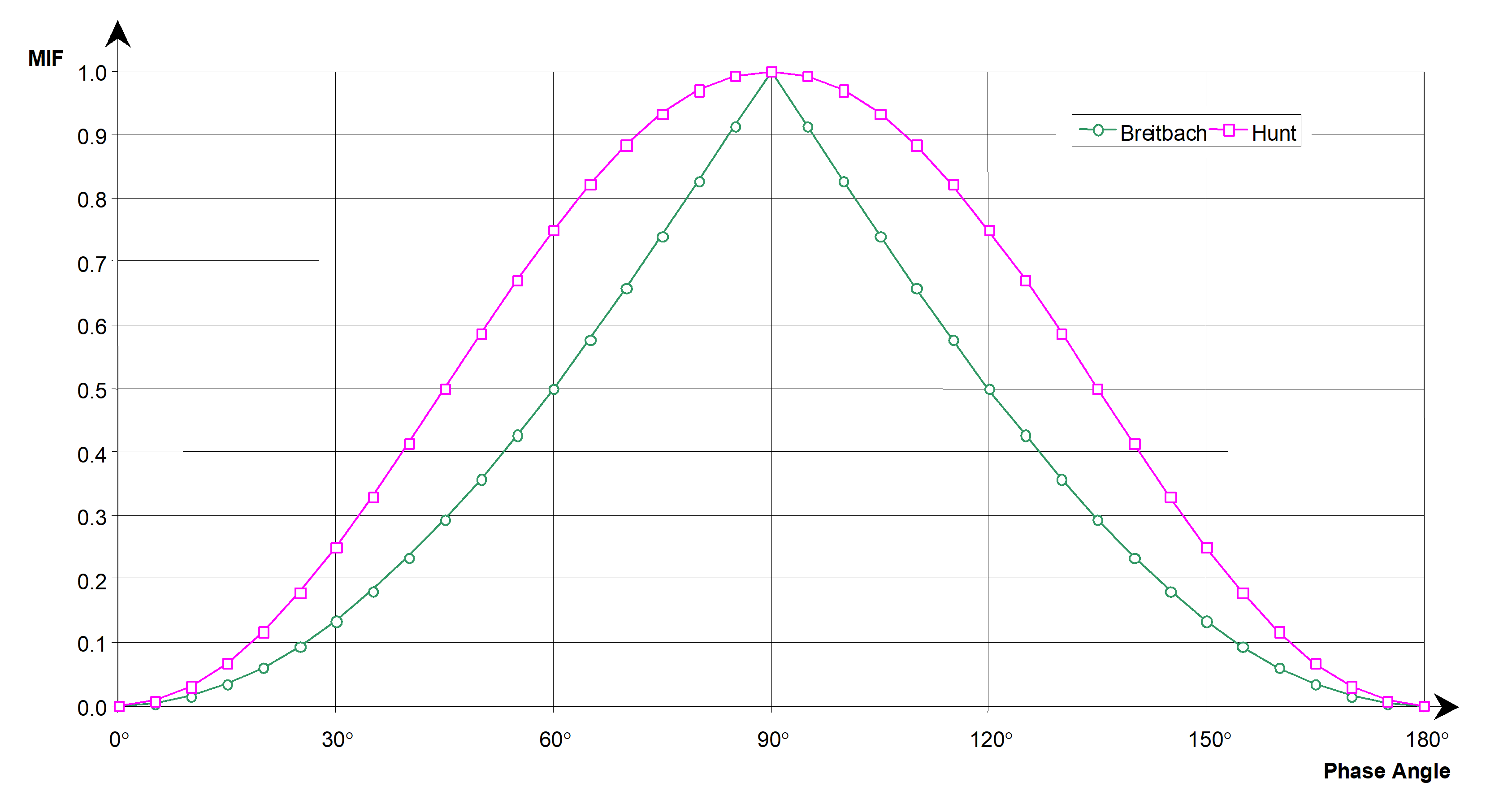  Figure 52: Comparison of mode indicator functions (MIF) according to Breitbach and Hunt

Auto­orthogonality

To perform the auto­orthogonality check, the measured mode shapes shall be transformed to the number of the analytical degrees of freedom.

This transformation can be facilitated if the measurement locations coincide as closely as possible with the finite element nodal points. The remaining nodal points can be conveniently determined by numerical interpolation. Consequently, a good measurement point plan takes into account the necessity of a reliable interpolation.

The off­diagonal elements shall be less than 10 %.

• 1    High off­diagonal values can indicate an inadequate isolation of the respective modes, especially if they are closely spaced in the frequency band, or if they are not very well tuned.
• 2    The degree of orthogonality of two measured modes with respect to the analytical mass matrix can be used as a criterion for the validity of the test results, for example to check the accuracy of the measurements and to detect duplicate modes.
• 3    The orthogonality can be highly dependent on the validity of the mass matrix (accuracy of TAM).

Modal assurance criterion

The modal assurance criterion compares the mode shape pattern directly without taking into account the mass distribution.

Two orthogonal modes do not always result in a zero MAC value.

Visual methods

The test set­up shall include hardware and software to enable the mode shapes to be visualized and animated.

A wire­frame model of the test article is frequently used for this purpose. The wire­frame model can be constructed by connecting the measurement points by line elements such that the contour of the test article is closely represented.

Generalized parameters

For each normal mode identified, the following parameters shall be determined:

• generalized mass;
• modal damping.
• 1    Since the generalized mass and the modal damping are related to each other via the latter, this cannot be done without measuring the exciter forces.
• 2    For the phase resonance method, modal damping can be determined from narrow­band frequency response measurements near the resonance. Proven evaluation methods are, for example,
• Nyquist circle curve fit,
• evaluation of real part slopes,
• complex power method, and
• forces in quadrate method.
• 3    The generalized parameters can be identified from the measured frequency response functions using suitable phase separation methods.
• 4    With the knowledge of the generalized parameters (natural frequencies, mode shapes, generalized masses and modal damping factors), the dynamic behaviour of the test article can be described using generalized coordinates.

Effective masses

For each normal mode identified, the effective masses related to the support point DOFs shall be determined.

• 1    Effective masses can be determined by adequate measurement of interface forces or by using the analytical mass matrix (see 3.2.13). However, measurement of the interface forces gives better results due to potential errors present in the analytical mass matrix.

• 2    The summation of all effective masses in each translatory and rotational direction yields the total structural mass and inertia, respectively. Therefore, the sum of the effective masses provides an indication of the completeness of the measured modes.

• 3    For structures with free­free boundary conditions, the following apply:

• the effective masses of the rigid body modes are equal to the total mass and inertia;

• the effective masses of the elastic modes are equal to zero.
  This criterion can be used to verify the quality of the elastic suspension.

• 4    The effective masses of clamped structures with fixed­free boundary conditions are related to the interface forces and moments.

Data storage and delivery

General aspects

The data exchange shall conform to the requirements specified in the test specification

For the test specification, see “Test specification” DRD in ECSS-E-ST-10-03.

Electronic data exchange should be used, employing established exchange formats.

• 1    For product exchange data, see ECSS-E-TM1020.
• 2    Usual data exchange formats are:
• For natural frequencies, mode shapes and modal damping: Universal File Format 55.
• For frequency response functions: Universal File Format 58.
  All data, regardless of the format, shall be accompanied by documentation containing a detailed description of the data, including the following:
• the format;
• date and status of data;
• the format of media (e.g. tape, back­up and operating system);
• the version of exchange format standard.

Test data storage

The modal survey test data shall be stored by the test facility for a period agreed with the customer.

The minimum storage time for test data in the European coordinated test facilities is 10 years.

Test­analysis correlation

Purpose

General

The experimental test modal data shall be compared with the analytical modal data, for the following purposes:

• To validate the mathematical model.
• To validate the test data.
• To select reliable test data for the mathematical model update.
• For taking corrective measures in a running test campaign.
• To detect erroneous areas in the mathematical model (error localization).

The correlation methods are given in Table 52.

Techniques identified as mandatory in Table 52 shall be applied.
Table 52: Most commonly used correlation techniques

Type	Techniques
Vector based techniques	-    Modal assurance criterion (MAC) a -    Orthogonality or cross-orthogonality a
DOF based techniques	-    Coordinate modal assurance criterion (CoMAC) -    Modulus difference a -    Coordinate orthogonality check
Frequency based techniques	-    Frequency difference a -    Frequency response assurance criterion (FRAC) -    Response vector assurance criterion (RVAC)
a    Mandatory (see 5.8.1.1b)

Mathematical model

The mathematical model shall describe the dynamic behaviour of the hardware in the frequency range of interest;
The mathematical model shall be applicable for coupling with other models for coupled static (with respect to I/F loads) and dynamic analysis;
The mathematical model shall describe the dynamic response in the frequency range of interest.

For the frequency range of interest, see 4.1.2.

Application of baseline correlation methods

As a minimum, the following steps shall be performed during the test analysis correlation:

• Selection of analysis DOFs: reduce the number of analysis mode shapes such that they are compatible with the experimental DOFs (number of accelerometers).

In general, the test modes have significantly fewer DOFs than the analysis mode shapes.

• Mode pairing: differentiate the mode pairs between analysis and test in order of the highest MAC or cross­orthogonality values, and calculate the eigenfrequency differences for these pairs.

For mode pairs not in the same order as the eigenfrequency sequence, the MAC can incorrectly indicate corresponding pairs.

• Cross­orthogonality: perform a general quality check of the FEM by means of the cross­orthogonality check. To perform the cross­orthogonality check specified in 5.8.1.3a.3, either the mass matrix shall be reduced to the number of the experimental DOFs, or the experimental mode shapes shall be expanded to the number of the DOFs of the FEM.

Criteria for mathematical model quality

Criteria for dynamic response predictions

The quality criteria for the test­analysis correlation shall ensure that the dynamic response predictions employing the test validated mathematical model conform to the accuracy requirements established by the customer.

Examples of test­analysis correlation quality criteria are given in Table 53.

Criteria for reduced mathematical models

Reduced mathematical models to be employed in dynamic response predictions shall represent the detailed FEM in conformance to the model quality criteria.

The usual reduced mathematical model quality criteria are given in Table 54 .

Conformance shall be demonstrated by comparing the dynamic behaviour of the reduced mathematical model with the dynamic analysis results obtained from the detailed FEM.
Table 53: Test-analysis correlation quality criteria

Item	Quality criterion a
Fundamental bending modes of a spacecraft	MAC:Eigenfrequency deviation:	> 0,9< 3 %
Modes with effective masses > 10 % of the total mass	MAC:Eigenfrequency deviation:	> 0,85< 5 %
For other modes in the relevant frequency range b	MAC:Eigenfrequency deviation:	> 0,8< 10 %
Cross­orthogonality check	Diagonal terms:Off­diagonal terms:	> 0,90< 0,10
Damping	To take measured values as input for the response analysis.To use realistic test inputs for this purpose.
Interface force and moment measurements	For modes with effective masses > 10 %: deviations of interface forces and moments < 10 %.
a     The quality criteria given are not normative and are given as examples for achieving a satisfactory test–analysis correlation. b     The relevant frequency range is, in general, determined by the launcher excitation spectrum up to 100 Hz. This frequency range can, however, be extended due to, for example, high frequency launcher dynamic excitations or specific requirements for AOCS control purposes.

Table 54: Reduced mathematical model quality criteria

Item	Quality criterion
Frequencies and modal masses of fundamental lateral, longitudinal and torsional modes	Effective mass: Eigenfrequency deviation:	< 5 %< 3 %
For other modes up to 100 Hz	Effective mass:Eigenfrequency deviation:	< 10 %< 5 %
Modes of reduced FEM (within frequency range of interest, see 4.1.2)	Total effective mass > 90 % of the rigid body mass.

Pre­test analysis

Purpose

Pre­test analyses shall be performed to support the modal survey test with respect to test planning and test execution.

• 1    The modal survey test is strongly supported by dynamic finite element analysis (FEA), for example modal analysis, response analyses and reduction of mathematical models, in order to optimize the output from the modal survey test.
• 2    The pre­test analysis requirements defined provide a general approach to FEA and improve the quality of modal survey test results. In particular, requirements for the following areas are given:
• Modal survey test FEM:        complete FEM;         test fixture participation.
• Test Analysis Model (TAM):        measurement point plan;        test predictions;         test fixture participation.
• 3    The pre­test analysis activities are shown in Figure 61.

Modal survey test FEM

Purpose

The modal survey test FEM shall represent the dynamic behaviour of the test article.

• 1    The FEM is applied to predict the modal survey test results (natural frequencies, vibration modes), to support the optimization of the exciter locations and the measurement point plan, and to assess the influence of adjacent structures (e.g. test fixtures).
  This FEM is often called the reference FEM and is a full (detailed) FEM.

• 2    For a detailed description of the reference FEM and the representation of the test article to be provided in the test prediction document, see clause 6.4.2.
  Figure 61: Modal survey pre­test analysis activities

Reduction of the detailed FEM

The reduced FEM shall represent the reference FEM in conformance with the criteria given in clause 5.8.2.2.

• 1    Usually the number of measurement points is (much) less than the total number of DOFs in the reference FEM. Therefore the size of the reference FEM is consistently reduced to match the number of measurement DOFs. The latter is equal to the number of measurement locations and the corresponding measurement directions (accelerometers).
• 2    The number, location and directions of the installed accelerometers define the size of the reduced FEM (number of retained or so-called dynamic DOFs). The remaining DOFs are mathematically eliminated from the total set of DOFs in the reference FEM.
• 3    In practice, the measurement point plan (number, locations, and directions of excitation and instrumentation) is usually defined with the aid of the reference or baseline FEM, where the predicted kinetic energy (KE) fraction is often used as an “accelerometer” location selector. DOFs with a relatively large KE are expected to dominantly influence the cross orthogonality matrix. Alternatively, the maximum linear independence criterion can be applied.
• 4    The reduced model is frequently called the test analysis model (TAM).
  The reduced FEM shall consist of a mass and stiffness matrix reduced to the number of measurement DOFs.

In general, the reduced mass and stiffness matrix are generated by applying a model reduction technique to the reference FEM. However, the TAM can also be a simplified FEM that adequately represents the reference model for test correlation and evaluation purposes.

The reduction of the reference FEM should be performed by employing one of the following techniques:
static reduction (Guyan);

dynamic reduction;

improved reduced system (IRS);

system equivalent reduction expansion process (SEREP).

• 1    The advantages and disadvantages of the most common model reduction techniques are summarized in Table 61.
• 2    The applicability of modal reduction techniques is limited because the physical DOFs are not preserved in the TAM. Model reduction based upon such techniques results in reduced mathematical models to be used for component mode synthesis (CMS) methods.
  Table 61: Advantages and disadvantages of model reduction techniques

Model reduction technique	Advantages	Disadvantages
Guyan (static) reduction	-    Easy to use and computationally efficient. -    Works well if A­set is properly defined. -    Available in most commercial FEA software.	-    Limited accuracy. -    Bad if A­set is badly defined. -    Unacceptable for high mass or stiffness ratio. -    Neglect of mass effects at omitted DOFs.
IRS	-    Better performance than Guyan (static) reduction. -    Takes into account the mass inertia effects associated with deleted DOFs.	-    No standard implementation into FEA software (e.g. Nastran). -    Errors if A­set is badly defined.
Dynamic reduction	-    Better performance than Guyan (static) reduction. -    Nearly exact structural response at any frequency.	-    No standard implementation into FEM software (e.g. Nastran). -    No obvious choice of eigenfrequency estimates. -    Limited experience.
SEREP	-    Exact reproduction of the lower natural frequencies of the full model. -    Possible to select specific modes to be included in reduction process.	-    No standard implementation into FEM software (e.g. Nastran). -    Limited experience.

Test analysis model (TAM)

Purpose

The TAM shall be used to scale measured vibration modes and to calculate the mass weighted cross orthogonality matrix between measured and analytical vibration modes.

For a detailed description of the TAM to be provided in the test prediction document, see clause 6.4.2.

The DOFs retained in the TAM shall:

• correspond one to one with accelerometers in the modal survey test configuration (location and measurement direction);
• coincide geometrically with the accelerometer locations for the modal survey test in the MPP in order to facilitate the correlation task.
• 1    For the MPP, see clause 6.3.3.
• 2    The TAM provides the basis for the test­analysis comparison.
• 3    The TAM has several major functions:
• The selection of the TAM DOFs supports the optimization of the test measurement and excitation locations.
• The reduced mass matrix provides a mean for performing on­site orthogonality checks of the test modes.
• The accuracy of the FEM during post­test correlation activities can be assessed and quantified in the form of orthogonality and cross­orthogonality checks.
• 4    The TAM is not considered to be suitable for the derivation of frequencies and mode shapes. As specified in 6.2.1, the FEM is used for this purpose.

TAM accuracy

The difference between the natural frequencies of the TAM and the “reference” model should be minimized in conformance with the quality criteria specified in Table 54.
The diagonal and off­diagonal terms of the cross orthogonality check between the TAM and “reference” model shall conform to the criteria given in Table 53.

The cross orthogonality check employs the mass matrix of the reduced model.

Measurement point plan (MPP)

The number of accelerometer locations (experimental DOFs) shall be chosen such that the modal characteristics of the test article (including natural frequencies, mode shapes, modal damping ratios, generalized and effective masses) in the frequency range of interest can be determined in conformance with the requirements listed in the test specification.

For the frequency range of interest, see 4.1.2. For the test specification, see “Test specification” DRD in ECSS-E-ST-10-03.

The accelerometer locations should be selected to ensure linear independence of the mode shapes of interest while retaining information about selected modal responses in the measurement data.

• 1    For the mode shapes of interest, see 4.1.2.
• 2    The following criteria can be applied in selecting the accelerometer locations:
• Retain DOFs with a large kinetic energy.
• Retain DOFs with a high mass­stiffness ratio.
• Retain DOFs that maximize the observability of mode shapes (effective independence).
• Remove only one DOF per iteration when optimizing the accelerometer locations with respect to kinetic energy and mass­stiffness ratio.
• 3    The suitability of the measurement locations can be assessed by evaluating the sensitivity of the predicted dynamic characteristics of the TAM with respect to the sensor locations. This can be done by using one of the following:
• The single (MIF) and multi­variate mode indicator function (MMIF) calculated from the reference FEM (not the TAM) response at the measurement DOFs.
• The AutoMAC calculated from the reference FEM modes at the measurement DOFs.

Test predictions

The test predictions shall be based upon both the reference FEM and the TAM.

The adequacy of the MPP and the TAM can be verified as follows:

• by exercising the identification procedure with the reference FEM and the MPP;
• by assessing the satisfactory performance of the data criteria (e.g. the cross­orthogonality checks results) by using the related TAM.
  The prediction model shall include the test article and test equipment.
• 1    E.g. adapters.
• 2    The results obtained enable the important modes to be determined based on the forcing function and load requirements, and the frequency range to be derived.

Test fixture participation

If test fixtures are applied during the modal survey test, these test fixtures shall be incorporated into the reference FEM and the TAM.
The influence of the test fixtures on the dynamic properties of the test article shall be determined.
The pure dynamic characteristics of the test article shall be extracted from the reference FEM after the influence of the test fixtures is removed.

In general, the reference FEM includes the test article and the test fixtures.

Documentation

FEM documentation

The reference FEM and the state of representation of the test article shall be described in the test prediction document in conformance with the “Test prediction” DRD in ECSS-E-ST-32.
The following items shall be reported, as a minimum:

• The supplier of the finite element software and the version number.
• The idealization of the hardware in the FEM.
• The description of the material properties.
• The CoG location.
• The rigid body mass matrix with respect to the CoG.
• The status of the analytical mass properties, i.e. whether estimated or measured.
• The standard FEM checks.
• The total number and the location or coordinates of the FEM DOFs.
• The boundary conditions applied.
• The natural frequencies.
• The normal mode shapes.
• The effective masses (in the case of fixed­free boundary conditions).
• The assumed damping values (amplification factors) as a function of the excitation frequency.
• The results of the response predictions.

For example, standard FEM checks are, for example, zero rigid body energy, free­free analysis (ideally 6 zero natural frequencies).

TAM documentation

The TAM shall be described in the “Test prediction” document in conformance with the “Test prediction” DRD in ECSS-E-ST-32.
As a minimum, the following information shall be provided:

• The general description of the TAM.
• The number and location or coordinates of the DOFs.
• The boundary conditions applied.
• The model reduction method.
• The CoG location.
• The rigid body mass matrix with respect to the CoG and comparison with the reference FEM.
• The standard FEM checks.
• The natural frequencies calculated with the TAM and comparison with the reference FEM.
• The effective masses calculated with the TAM and comparison with the reference FEM.
• The results of MAC matrix calculation correlating the TAM mode shapes with the reference FEM.

ANNEX(informative) Excitation signals

Overview

The main characteristics of the excitation signals most commonly used for modal testing purposes are presented in this annex. Detailed descriptions can be found in the sources of information given in Annex D.

Purpose and classification

Purpose of excitation

The application of a dynamic excitation to the structure is an essential part of the modal survey test. The excitation causes vibrations of the structure in the frequency range of interest (see 4.1.2) such that the applied dynamic forces and the corresponding structural responses can be adequately measured.

The excitation can be applied at a single location in the structure or simultaneously at multiple locations.

The excitation signals used are large enough to provide measurement signals which are sufficiently above the measurement noise level.

Commonly used excitation signals

A classification of the most common dynamic excitation signals is given in Figure A-1.

Selection of the excitation signal

Excitation signals are selected according to the following criteria:

availability and complexity of the equipment;

available time frame for the testing;

potential non­linearity of the test structure;

controllability of the excitation signal;

sensitivity of the signal for bias and variance errors;

definition of measurement accuracy.

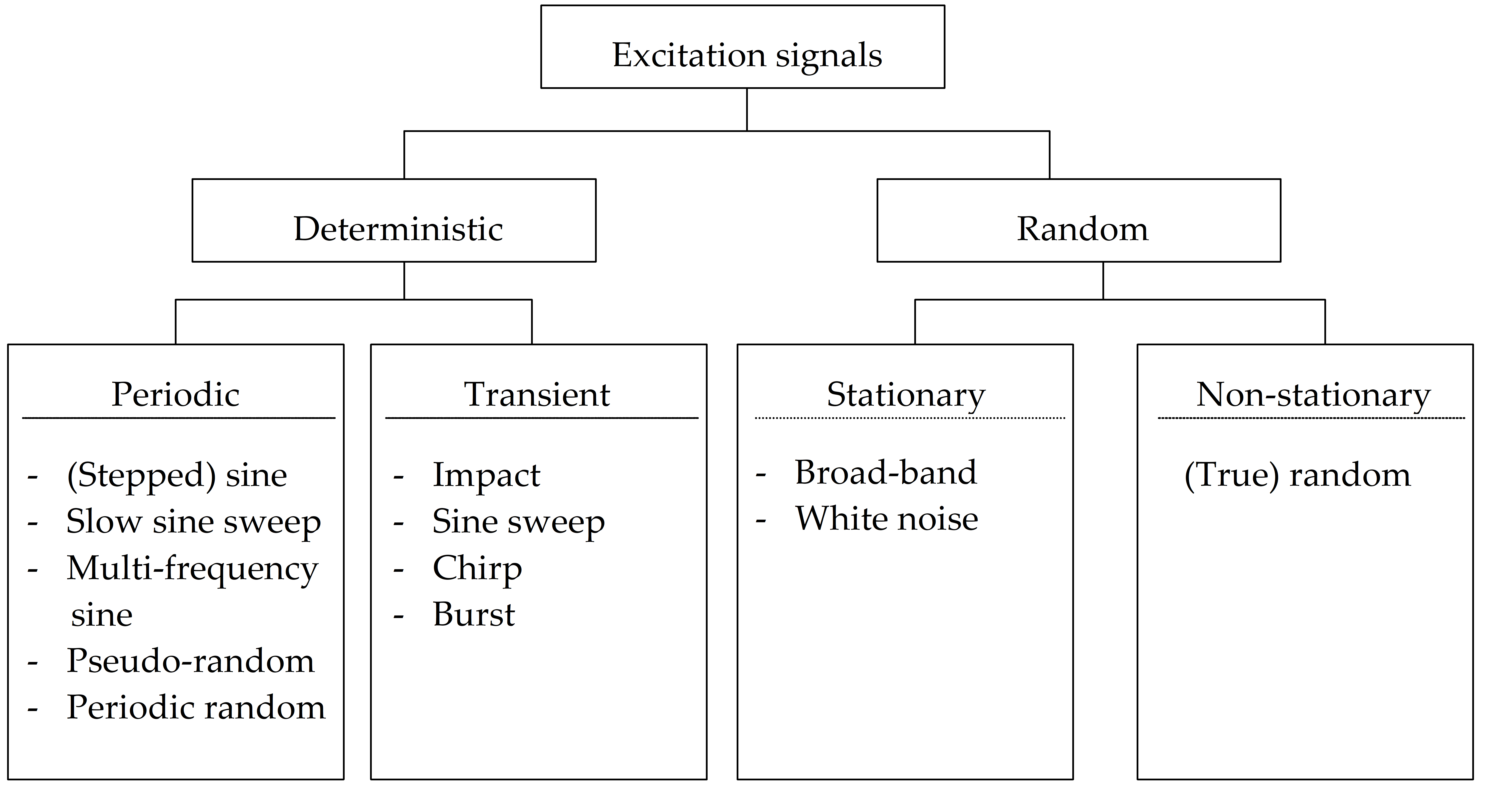Figure: Classification of common excitation signals

Excitation methods

Impact

The impact signal is a transient deterministic signal and consists of a pulse only applied during a very short part of the total modal data acquisition period. The shape, width and amplitude of the pulse determine the frequency content of the excitation force spectrum.

It is good practice not to apply the impact excitation method to non­linear structures since the excitation force cannot be controlled and repeated measurements can be affected by the non­linear behaviour of the structure.

Pure random

The pure random signal is a non­periodic stochastic signal containing all frequencies in a specified frequency range.

Pseudo­random

The pseudo­random signal is an excitation signal in which the frequency spectrum consists only of integer multiples of the discrete Fourier transform frequency increment.

The periodicity of the pseudo­random signal avoids leakage problems.

Periodic random

The periodic random signal consists of discrete frequencies at integer multiples of the frequency resolution used by the discrete Fourier transform (similar to pseudo­random signal). It has a random magnitude and phase content.

The structure is repeatedly excited with the same time block until the transient responses have died out and a steady­state condition is reached. The input and response signals are then recorded as one average.

The periodicity of the periodic­random signal with respect to the observation window ensures that leakage problems are avoided.

Periodic chirp

The periodic chirp signal is a very rapid sine sweep where the frequency is swept up and down in one observation period of the data acquisition. This sweeping is repeated in the procedure such that it becomes a periodic function.

The periodic chirp signal is a special case of a pseudo­random signal and therefore has similar characteristics.

Burst excitation

Burst excitation signals are transients consisting of a short section of a continuous signal (e.g. sine wave, sine sweep, and random) followed by a zero output section. The resulting response shows a transient build­up followed by a decay. The section length after which the signal drops to zero depends on the damping of the test structure.

Swept sine

The swept sine signal is a sine excitation signal with a continuously varying frequency. Usually a linear or logarithmic type of sweep rate is applied. In a strict sense the swept sine is a transient excitation. Therefore, measuring virtually steady­state response characteristics can be assumed only if a sufficiently slow sweep rate is selected.

To ensure that the measured magnitude of the motion response is within 5 % of the steady state value, ISO 7626-2 prescribes maximum linear and logarithmic sweep rates as follows:

Linear sweep:         (Hz/min).

Logarithmic sweep:     (oct/min).

Swept sine excites the test structure for each measurement at virtually one frequency and therefore yields a signal with the best signal to noise, and peak to RMS, ratios.

Swept sine is ideally suited for characterizing non­linear systems since the amplitude and frequency can be very precisely controlled.

Stepped sine

The stepped sine excitation consists of step-wise changing frequencies applied sequentially. At each frequency the excitation is applied over a small interval of time. Therefore, steady­state response conditions can only be achieved if the length of the time interval is sufficiently long.

Digital signal processing provides varying frequency spacing, yielding data condensation and testing time reduction.

Stepped sine has the same excellent signal to noise and peak to RMS ratios and the same properties with respect to non­linearities as the swept sine excitation signal.

ANNEX(informative) Estimation methods for modal parameters

Overview

The main characteristics of estimation methods for modal parameters are presented in this annex. Detailed descriptions can be found in the sources of information given in Annex D and in Bibliography.

Theoretical background and overview

Description of linear mechanical systems

The equations of motion of a linear, time invariant mechanical system with viscous type damping are given in matrix notation by


Equation (C -1)

where

[M], [C] and [K] are the physical mass, damping and stiffness matrices, respectively;

{f(t)}     is the time­dependent excitation vector;

{x(t)}     is the vector of physical displacements.

By means of the modal transformation

 where 

Equation (C -2)

the physical coordinates are described by the real normal mode shapes {}k of the undamped system and the generalized coordinates qk(t).

Introducing equation (C-2) into equation (C-1) and pre­multiplying with the transposed modal matrix {}T yields the equivalent modal formulation:


Equation (C -3)

where [m], [c] and [k] are the generalized mass, damping and stiffness matrices, respectively.

These matrices are diagonal matrices due to the orthogonality relation of the real normal modes of undamped systems and the assumption of proportional damping. F(t) is the generalized excitation vector.

The modal transformation reduces the number of physical degrees of freedom to the number of modal degrees of freedom, which is the number of modes in the frequency range of interest (see 4.1.2).

Usually, the generalized damping matrix [c] is a non­diagonal matrix, for most practical applications, however, proportional damping characteristics can be assumed for the structure resulting to a diagonal damping matrix.

Classification of commonly used modal parameter estimation methods

Overview

The modal parameter estimation methods provide the mathematical tools for determining the basic modal characteristics from the measured frequency response functions or measured time histories:

Natural frequency         fr =  r /2

Mode shapes        {}r

Modal damping ratio     r

Modal parameters is usually estimated by selecting the parameters of an appropriate modal model such that the measured frequency responses or time histories are sufficiently approximated by the modal model.

In addition to the basic modal parameters fr, {}r and r there are several methods for providing estimates of the modal participation factors {L}r and residue vectors {A}r.

Usually, modal parameters are considered to be global properties of the system, i.e. there is only one answer for each modal parameter. Most modal parameter estimation methods provide estimates for the modal frequencies and the modal damping in a global sense but only a few provide estimates for the mode shapes in a global sense.

The modal parameter estimation process involves a greatly over­determined problem. In general, modal parameter estimates using different methods are not the same due to differences in the following:

the modal model and the model domain (time, frequency or spatial);

the way in which the measured data is used in the methods and weighting factors applied to this data;

the experience of the user.

Table B-1  provides an overview and classification of most commonly used modal parameter estimation methods; this overview is not exhaustive.

Time or frequency domain methods

The advantages and disadvantages for time and frequency domain methods are presented in Table B-2.

Single or multiple degree of freedom methods

The advantages and disadvantages of single (SDOF) and multiple degree of freedom (MDOF) methods are presented in Table B-3.

The SDOF methods have been developed and used in the very early days of modal testing.

SDOF methods are based on the modal model in the frequency domain and provide local estimates for the system poles (natural frequency and damping) and complex (or real) modal vectors.

Other aspects of selecting a modal parameter estimation method

In addition to the time or frequency domain methods, and SDOF or MDOF methods, the additional aspects that are usually considered in selecting an appropriate modal parameter estimation method, include for example

modal or direct model identification,

real or complex mode shapes, and

global or local parameter estimation.

An overview is given in Table B-4.

Table: Overview and classification of commonly used modal parameter estimation methods

Method	SDOF or MDOF	Local or global estimate	Single or multiple inputs	Modal or direct model	Time or Frequency domain	Poles or mode shapes	Real or complex modes
Peak picking	SDOF	Local	Single	Modal	F	p
Mode picking	SDOF	Local	Single	Modal	F	ms	Real or complex
Circle fit	SDOF	Local	Single	Modal	F	p and ms	Real or complex
ITD	MDOF	Global	Multiple	Modal	T(first order)	p and ms	Complex
LSCE	MDOF	Global	Single	Modal	T(high order)	p
PTD (PRCE)	MDOF	Global	Multiple	Modal	T(high order)	p
ERA	MDOF	Global	Multiple	Direct	T(first order)	p and ms	Complex
Non­linear LSFD	MDOF	Global	Multiple	Modal	F	p and ms	Real or complex
PolyMAX	MDOF	Global	Multiple	Modal	F	p and ms	Real or complex
ISSPA	MDOF	Global	Multiple	Direct	F	p and ms	Real
OPM	MDOF	Global	Multiple	Modal	F	p and ms	Real or complex
FDPI	MDOF	Global	Multiple	Direct	F	p and ms	Real or complex
SFD	MDOF	Global	Single	Modal	F	p and ms	Real or complex
CMIF	MDOF	Global	Multiple	Modal	F	p and ms	Real or complex
ITD:     Ibrahim time domain method LSCE:    Least squares complex exponential PTD:     Polyreference time domain method PRCE:     Polyreference complex exponential ERA:     Eigensystem realization algorithm LSFD:     Least squares frequency domain				Poly:     Polyreference modal analysis extended ISSPA:    Identification of structural system parameters OPM:     Orthogonal polynomial method FDPI:     Frequency domain direct parameter identification SFD:     Simultaneous frequency domain CMIF:     Complex mode identification function

Table: Advantages and disadvantages of the time and frequency domain methods

Domain	Modal parameter estimation	Advantages	Disadvantages
Time	Based on the direct use of the time histories of the excitation (input) and the response (output) signals.	-    Best results when large frequency range or large number of modes exist in the acquired data. -    Better numerical conditioning than frequency domain equivalents. -    Better adapted to lightly damped systems (long usable time signal). -    Avoidance of signal processing errors. -    Broad­band analyses. -    Unique qualities to enable modal identification from responses obtained during operation.	-    Residual effects of modes located outside the frequency range of analysis not taken into account. -    Time domain methods excluded if available FRF do not have equal frequency spacing (inverse FFT cannot be performed). -    Only estimates of modes inside the frequency range of analysis provided.
Frequency	Based on frequency response functions for one of the following: -    single input­output relations Hij(j); -    the complete assembly of input­output relations, i.e. the entire FRF matrix H(j.	-    Best results when frequency range of interest (see 4.1.2) is limited or the number of modes is relatively small. -    Approximation of effects of out­of­band modes, in particular concerning mode shape estimation (residual effects). -    Better adapted to highly damped systems (large number of relevant sampling points at resonance peaks). -    More convenient interpretation of structure response properties by inspecting the frequency response functions rather than time domain impulse response functions.	-    Numerical conditioning worse than time domain equivalents. -    Effect of frequency powers unfavourable for broad­band analyses. -    Specific problems concerning frequency resolution, leakage and high modal densities.

Table: Advantages and disadvantages of single and multiple degree of freedom methods

SDOF or MDOF	Approach	Advantages	Disadvantages
SDOF	Separate evaluation of each mode in the frequency range of interest (see 4.1.2) assuming the following: -    only one mode is important in a given frequency range; -    modal parameters for this mode can be determined independently of the other modes.	-    Very simple to use and fast method for only very few modes. -    Can be performed with little computational effort and memory. -    Can be performed without reduction of the system under investigation to SDOF system, since all modes in the frequency range of interest (see 4.1.2) are analyzed sequentially, one after the other. -    Particularly valuable tool for quick look purposes (e.g. in the preliminary phases of modal tests or where quick estimates of the basic dynamic characteristics of a structure are performed).	-    Not applicable to separation of closely spaced modes. -    Can become time­consuming when large number of modes and their modal parameters are analyzed.
MDOF	General case in which: -    several or all modes are included in the modal model; -    the modal parameters of these modes are determined simultaneously.	-    Better than SDOF methods as it is based on more complete models of the dynamic system. -    As a result, MDOF methods provide in general more reliable results than SDOF methods.	-    Cannot be carried­out without personnel with a significant background knowledge. -    Relatively long times for data processing.

Table: Other aspects of selecting a modal parameter estimation method

Purpose	Method	Characteristics
Modal or direct model identification	Modal	-    Output signals are described as linear combinations of characteristic solutions (the system modes) of the differential equations of motion. -    Subsequently, the unknown parameters and the modal parameters, are estimated.
	Direct	-    Modal parameters are estimated directly from the differential equations of motion rather than characteristic solutions. -    1st step: estimation of the coefficients of the input­output differential equations. -    2nd step: calculation of the desired modal parameters from these coefficients, for example, by determining the eigenvalues of the estimated mass, stiffness and damping matrices.
Real or complex mode shapes	Real	Real mode shapes: -    exist for undamped systems; or -    can be adequately computed from complex modes of proportionally damped systems.
	Complex	Complex mode shapes exist for non­proportionally damped systems.
Local or global parameter estimation	Local	-    The dependency of the poles, mode shape coefficients and modal participation factors from either the input or output location, or both, is taken into account. -    Measurement data from each measurement point are processed simultaneously.
	Global	Single­input, single­output measurement data are used for the eigenvalue computation, i.e. one response function at a time.

Frequency domain methods

Single degree of freedom (SDOF) methods

Peak picking

Peak picking provides local estimates for the system poles (natural frequency and damping). Only real mode properties can be deduced with this method.

The method is based on the fact that the FRF has extreme values around the natural frequencies.

The method provides a good estimate for the damped natural frequency r. The corresponding damping ratio r can be estimated from the half power bandwidth frequencies:

Peak picking provides adequate estimates for structures where the FRF exhibits well­separated modes, and where the extremes of either light or very strong damping are not present.

Mode picking

Mode picking provides local estimates for complex (or real) modal vectors.

The FRF value at r provides an estimate of the residue or mode shape coefficient if multiplied by the modal damping r. An estimate of r is done in order to apply the mode picking technique.

Circle fitting

Circle fitting provides local estimates for complex (or real) modal vectors.

The method is based on the fact that the FRF of a SDOF system (in terms of velocity or force) describes a circle in the complex plane (Nyquist plot).

It is good practice to use the receptance form of the FRF in the case of structural damping and the mobility form in the case of viscous damping to construct the Nyquist plot.

The damped natural frequency r is derived in one of the following ways:

the point at which the maximum rate of change of angle between data points in the complex plane (maximum angular spacing) occurs;

the frequency of the data point at which the phase angle is closest to the phase angle of the centre of the circle.

The difference is negligible for well separated modes.

The damping ratio r is estimated from the half power bandwidth frequencies frequency  and .

This method is fast but can produce erroneous results, mainly close to nodal points of modes, in the absence of user interactions.

Multiple degree of freedom (MDOF) methods

Non­linear, least squares frequency domain method (LSFD)

The LSFD method generates global estimates for the system poles, mode shapes and modal participation factors (if applied for multiple input).

The LSFD method is based upon the modal model in the frequency domain.

The LSFD method provides an FRF approximation between the response and input locations within the frequency range of interest (see 4.1.2). The effects of modes below or above the frequency range of interest are taken into account by residual terms.

The unknown FRF parameters are determined by minimizing the global error between the measured and the estimated FRF. Since this set of equations is highly non­linear in the unknowns, the problem is solved iteratively in a linearized manner around a modal model with initial estimates for the unknown parameters.

Although the LSFD method has the classical disadvantages of iterative procedures (e.g. performance depending on the initial estimates of all unknowns, the limited convergence speed, the risk of divergence and inappropriate application due to limited user experiences and skills), it can be a useful tool for improving the accuracy of an already fairly reliable modal model.

The complexity of the LSFD method can be significantly improved if the system poles and the modal participation factors have already been estimated by other methods (e.g. polyreference least squares complex exponential) since then the global error functional becomes a linear set of equations in the remaining unknowns, i.e. the modal displacements and the residual terms.

Identification of structural system parameters (ISSPA)

The ISSPA method identifies a high order incomplete direct model from multiple input - multiple response measurement data. The method aims at providing global estimates for the system poles and the normal mode shapes.

The ISSPA method cannot be applied unless there are at least as many response locations as modes selected for identification.

The mass modified stiffness matrix defines an eigenvalue problem yielding the system’s natural frequency and normal mode shapes.

Proportional damping values are estimated from the mass modified damping matrix.

Disadvantages of the ISSPA method are:

information on the modal participation factors is not provided;

the damping estimate can be inaccurate in the case of “noisy” data.

Frequency domain direct parameter identification (FDPI)

The FDPI method identifies a low order complete direct model from multiple input - multiple output FRF measurements. It provides global estimates for the system poles, the mode shapes and the modal participation factors.

The FDPI method is performed in two steps:

Estimate the system matrices.

Derive the system poles, the mode shapes and the modal participation factors from the estimated system matrices.

The FDPI method includes significant data reduction, based upon the selection of “independent” response locations, to obtain a complete model. This process, however, demands user interaction and experience.

Complex mode indicator function (CMIF)

The CMIF is a spatial domain technique that indicates the existence of real normal or complex modes and the relative magnitude of each mode. It is a multiple reference method.

The CMIF provides global estimates for the damped natural frequencies (however limited by the accuracy of the frequency resolution) and the corresponding unscaled mode shapes.

Advantages of the CMIF are:

very simple to use as it is, essentially, a SDOF method;

very fast and therefore excellent for obtaining initial estimates, and relatively insensitive to noise.

Disadvantages of the CMIF are:

in general, only modes which are relatively uncoupled are extracted;

modes can be wrongly indicated since noise, leakage, non­linearity, and cross eigenvalue effects can create peaks in the CMIF plot.

Polyreference modal analysis extended (PolyMAX)

The PolyMAX method is a least­squares frequency­domain method using multiple input - multiple output frequency response functions as primary data. Basically, the method is a further evolution of the least squares complex frequency domain (LSCF) method.

The PolyMAX method can be implemented in a very similar way to the polyreference (time­domain) LSCE method:

Construct a stabilization diagram containing frequency, damping and modal participation information.

Determine the mode shapes by a least­squares approach, based on the user selection of stable poles.

Advantages of the PolyMAX method are:

Very stable identification of the system poles and modal participation factors as a function of the specified system order, leading to “easy to interpret” stabilization diagrams (to detect and eliminate computational noise modes).

Potential for automating the parameter estimation process and to apply it to “difficult” estimation cases such as high­order or highly damped systems with large modal overlap.

Time domain methods

Basics

The time domain modal identification methods are based on the direct use of a structure’s free decay time function or impulse response function to determine the modal parameters. These methods are known as complex exponential (CE) methods where it is assumed that the response function (displacement, velocity or acceleration) can be expressed as a linear combination of damped complex exponential components containing the system eigensolutions (eigenvalues and mode shapes):

All methods are multiple degree of freedom (MDOF) methods and are based on an auto­regressive moving average (ARMA) model.

Application of the complex exponential methods to impulse response functions yields properly scaled modal parameters that can be used for generalized mass and stiffness calculations. This is not the case for free decay responses.

Ibrahim time domain method (ITD)

The ITD method is a multi­curve, time domain analysis method with a single reference (input). The main objective of the ITD is to obtain a unique set of modal parameters from a set of free vibration measurements in a single analysis, i.e. processing all the measured data at once.

The ITD method uses a low order homogeneous model to describe the system.

Specific advantages of the ITD are:

It is applicable to any measured free vibration data whether or not the excitation forces are available.

Usually, a minimum amount of time data is used and therefore the method is well suited for analyzing short time transients.

Global estimates of eigenvalues and mode shapes are performed in one computational step with excellent numerical conditioning.

Disadvantages of the ITD are:

Due to it being a single reference method, repeated or pseudo­repeated roots cannot be handled.

It has a tendency to generate a large number of “computational” modes. However, several methods and procedures are available to reduce or exclude “computational” modes, for example, by the modal confidence factor.

Least squares complex exponential method (LSCE)

The LSCE method is a single reference method. A consistent set of global parameters is obtained from different impulse response functions such as overcoming the variations with standard CE methods.

Processing of the several impulse response functions occurs simultaneously.

Disadvantages of the LSCE are:

Due to it being a high order algorithm, more time domain data is used compared to low order algorithms (e.g. ITD or ERA).

Limitations exist for cases involving high damping.

Polyreference time domain method (PTD)

The PTD method is a consistent extension to the LSCE method. It enables multiple references to be included and as such the ability to resolve close modal frequencies is enhanced.

To determine the modal parameters, the PTD uses a set of free decay responses or impulse response functions that are excited by multiple initial conditions or from multiple exciter locations.

It is good practice to make initial investigations of the influences of non­linearities and noise since the method is particularly sensitive to non­linear responses for free decay testing.

The PTD method provides global estimates of both the eigenvalues and the modal participation factors. Mode shapes are estimated by curve fitting in the time or frequency domain. Residual terms can be included when curve fitting is performed in the frequency domain.

Disadvantages of the PTD method are identical to those of the LSCE (see B.4.3).

Eigenvalue realization algorithm (ERA)

The ERA algorithm is based upon state­space theory using controllability and observability concepts. Similarities with the PTD method exist since multiple input excitation cases can be handled and repeated roots identified. However, other than for the PTD, a low order ARMA model is used resulting to large matrix sizes.

The ERA makes extensive use of accuracy indicators to assess the effects of noise and non­linearities, for example:

rank of the block data matrix formulated from damped complex exponential functions;

modal amplitude coherence;

modal phase collinearity.

As for the PTD, it is good practice to make initial investigations of the influences of non­linearities and noise since the method is particularly sensitive to non­linear responses for free decay testing.

The ERA method is particularly well suited to on­orbit modal testing and identification applications.

Disadvantages of the ERA method are:

It has a tendency to generate a large number of “computational” modes in the frequency range being selected for modal identification.

It has a limited applicability unless large computation capability (memory) is available to solve problems with a large number of response sensors (typical for low order methods).

ANNEX(informative) Modal test - mathematical model verification checklist

Table C-1 presents the verification checklist for mathematical models of the test set­up (the test article and, where relevant, for the modal survey test prediction, the test adapter) that has been generated with the purpose of supporting the modal survey test predictions and the test execution.

Table: Verification checklist for mathematical models supporting modal survey tests

Identifier	Description
C.1	General payload information
C.2	Payload description and characteristics
C.3     C.3.1     C.3.2     C.3.3     C.3.4     C.3.5         C.3.5.1         C.3.5.2     C.3.6     C.3.7     C.3.8     C.3.9	Modal test information -    Test facility, dates, point of contact -    Summary of tests -    Reference documents -    Test article description -    Test boundary conditions         Constrained         Free­free -    Test instrumentation, equipment and software -    Excitation methods -    Linearity checks -    Test modal analysis activities
		C.4     C.4.1     C.4.2	Description of analytical model -    Flight analytical model for verification loads analysis -    Test­analysis model for correlation analysis (TAM)
				C.5	Test analytical model adjustments
				C.6     C.6.1     C.6.2     C.6.3     C.6.4         C.6.4.1         C.6.4.2         C.6.4.3         C.6.4.4         C.6.4.5     C.6.5     C.6.6     C.6.7     C.6.8	TAM - test data correlation -    Data summary, frequency comparisons, mode shape descriptions -    Test fixture participation -    Forced response test model - TAM comparisons -    Quantitative comparisons of mode shapes         Kinetic energy         Modal scale factor         Modal assurance criterion         Effective modal mass         Cross­orthogonality check -    Qualitative comparison of mode shapes -    Unique (uncorrelated) modes -    Analysis methodology and software -    General comments

ANNEX(informative) References

Braun, 2001 Encyclopedia of Vibration (1st Ed.), S. Braun et al., Academic Press Ltd., 2001; ISBN 0122270851

Ewins, 2000 Modal Testing – Theory, Practice and Application (2nd Ed.), D.J. Ewins, Research Studies Press Ltd., 2000; ISBN 0863808184

Heylen, 1997 Modal Analysis Theory and Testing, W. Heylen, St. Lammens & P.Sas, Publication Katholieke Universiteit Leuven (PMA), 1997

Friswell, 1995 Finite Element Model Updating in Structural Dynamics, M.I. Friswell & J.E. Mottershead Kluwers Academic Publishers, 1995; ISBN 0792334310

Døssing, 1987 Structural Testing, O. Døssing Part 1: Mechanical Mobility MeasurementsPart 2: Modal Analysis and Simulation Brüel & Kjær Publication, April 1987

Maia, 1998    Theoretical and Experimental Modal Analysis, N.M.M. Maia & J.M.M. Silva Research Studies Pres Ltd., 1998; ISBN 0863802087

DTA Handbook on Guidelines to Best Practice, Dynamic Testing Agency Vol. 3: Modal Testing

Bibliography

ECSS-S-ST-00	ECSS system – Description, implementation and general requirements
ECSS-Q-ST-40	Space product assurance – Safety
ECSS-E-TM-10-20	Space engineering – Product data exchange
ISO 7626-2	Vibration and Shock - Experimental Determination of Mechanical Mobility - Part 2: Measurements Using Single­point Translation Excitation with an Attached Vibration Exciter