Space engineering

Control performance

Foreword

This Standard is one of the series of ECSS Standards intended to be applied together for the management, engineering and product assurance in space projects and applications. ECSS is a cooperative effort of the European Space Agency, national space agencies and European industry associations for the purpose of developing and maintaining common standards. Requirements in this Standard are defined in terms of what shall be accomplished, rather than in terms of how to organize and perform the necessary work. This allows existing organizational structures and methods to be applied where they are effective, and for the structures and methods to evolve as necessary without rewriting the standards.

This Standard has been prepared by the ECSS-E-ST-60-10 Working Group, reviewed by the ECSS Executive Secretariat and approved by the ECSS Technical Authority.

Disclaimer

ECSS does not provide any warranty whatsoever, whether expressed, implied, or statutory, including, but not limited to, any warranty of merchantability or fitness for a particular purpose or any warranty that the contents of the item are error-free. In no respect shall ECSS incur any liability for any damages, including, but not limited to, direct, indirect, special, or consequential damages arising out of, resulting from, or in any way connected to the use of this Standard, whether or not based upon warranty, business agreement, tort, or otherwise; whether or not injury was sustained by persons or property or otherwise; and whether or not loss was sustained from, or arose out of, the results of, the item, or any services that may be provided by ECSS.

Published by:     ESA Requirements and Standards Division
    ESTEC, P.O. Box 299,
    2200 AG Noordwijk
    The
Copyright:     2008 © by the European Space Agency for the members of ECSS

Change log

ECSS-E-ST-60-10A	Never issued
ECSS-E-ST-60-10B	Never issued
ECSS-E-ST-60-10C 15 November 2008	First issue

Introduction

This standard focuses on the specific issues raised by managing performance aspects of control systems in the frame of space projects. It provides a set of normative definitions, budget rules, and specification templates applicable when developing general control systems.

The standard is split up in two main clauses, respectively dealing with:

Performance error indices and analysis methods.

Stability and robustness specification and verification for linear systems.

This document constitutes the normative substance of the more general and informative handbook on control performance, issued in the frame of the E-60-10 ECSS working group. If clarifications are necessary (on the concepts, the technical background, the rationales for the rules for example) the readers should refer to the handbook.

It is not intended to substitute to textbook material on automatic control theory, neither in this standard nor in the associated handbook. The readers and the users are assumed to possess general knowledge of control system engineering and its applications to space missions.

Scope

This standard deals with control systems developed as part of a space project. It is applicable to all the elements of a space system, including the space segment, the ground segment and the launch service segment.

It addresses the issue of control performance, in terms of definition, specification, verification and validation methods and processes.

The standard defines a general framework for handling performance indicators, which applies to all disciplines involving control engineering, and which can be applied as well at different levels ranging from equipment to system level. It also focuses on the specific performance indicators applicable to the case of closed-loop control systems – mainly stability and robustness.

Rules are provided for combining different error sources in order to build up a performance error budget and use this to assess the compliance with a requirement.

• 1    Although designed to be general, one of the major application field for this Standard is spacecraft pointing. This justifies why most of the examples and illustrations are related to AOCS problems.
• 2    Indeed the definitions and the normative clauses of this Standard apply to pointing performance; nevertheless fully specific pointing issues are not addressed here in detail (spinning spacecraft cases for example). Complementary material for pointing error budgets can be found in ECSS-E-HB-60-10.
• 3    For their own specific purpose, each entity (ESA, national agencies, primes) can further elaborate internal documents, deriving appropriate guidelines and summation rules based on the top level clauses gathered in this ECSS-E-ST-60-10 standard.
  This standard may be tailored for the specific characteristic and constrains of a space project in conformance with ECSS-S-ST-00.

Normative references

The following normative documents contain provisions which, through reference in this text, constitute provisions of this ECSS Standard. For dated references, subsequent amendments to, or revision of any of these publications do not apply, However, parties to agreements based on this ECSS Standard are encouraged to investigate the possibility of applying the more recent editions of the normative documents indicated below. For undated references, the latest edition of the publication referred to applies.

ECSS-S-ST-00-01

ECSS System – Glossary of terms

Terms, definitions and abbreviated terms

Terms from other standards

For the purpose of this Standard, the terms and definitions from ECSS-S-ST-00-01 apply, in particular for the following terms:

error

performance

uncertainty

Terms specific to the present standard

absolute knowledge error (AKE)
instantaneous value of the knowledge error at any given time

• 1    This is expressed by:    

• 2    See annex A.1.3 for defining requirements on the knowledge error.
  absolute performance error (APE)
  instantaneous value of the performance error at any given time

This is expressed by:    

error index
parameter isolating a particular aspect of the time variation of a performance error or knowledge error

• 1    A performance error index is applied to the difference between the target (desired) output of the system and the actual system output.
• 2    A knowledge error index is applied to the difference between the actual output of the system and the known (estimated) system output.
• 3    The most commonly used indices are defined in this chapter (APE, RPE, AKE etc.). The list is not limitative.
  individual error source
  elementary physical characteristic or process originating from a well-defined source which contributes to a performance error or a performance knowledge error

For example sensor noise, sensor bias, actuator noise, actuator bias, disturbance forces and torques (e.g. microvibrations, manoeuvres, external or internal subsystem motions), friction forces and torques, misalignments, thermal distortions, assembly distortions, digital quantization, control law performance (steady state error), jitter, etc.

knowledge error
difference between the known (estimated) output of the system and the actual achieved output

• 1    It is denoted by eK.

• 2    Usually this is time dependent.

• 3    Sometimes confusingly referred to as “measurement error”, though in fact the concept is more general than direct measurement.

• 4    Depending upon the system, different quantities can be relevant for parameterising the knowledge error, in the same way as for the performance error. A degree of judgement is used to decide which is most appropriate.

• 5    For example: the difference between the actual and the known orientation of a frame can be parameterised using the Euler angles for the frame transformation or the angle between the actual and known orientation of a particular vector within that frame.
  mean knowledge error (MKE)
  mean value of the knowledge error over a specified time interval

• 1    This is expressed by:         

• 2    See annex A.1.4 for discussion of how to specify the interval t, and annex A.1.3 for defining requirements on the knowledge error.
  mean performance error (MPE)
  mean value of the performance error over a specified time interval

• 1    This is expressed by:    

• 2    See annex A.1.4 for discussion of how to specify the interval .
  performance drift error (PDE)
  difference between the means of the performance error taken over two time intervals within a single observation period

• 1    This is expressed by:    

• 2    Where the time intervals t1 and t2 are separated by a non-zero time interval tPDE.

• 3    The durations of t1 and t2 are sufficiently long to average out short term contributions. Ideally they have the same duration. See annex A.1.4 for further discussion of the choice of t1 , t2, tPDE.

• 4    The two intervals t1 and t2 are within a single observation period
  performance error
  difference between the target (desired) output of the system and the actual achieved output

• 1    It is denoted by eP.

• 2    Usually this is time dependent.

• 3    Depending upon the system, different quantities can be relevant for parameterising the performance error. A degree of judgement is used to decide which is most appropriate.

• 4    For example: The difference between the target and actual orientation of a frame can be parameterised using the Euler angles for the frame transformation or the angle between the target and actual orientation of a particular vector within that frame.
  performance reproducibility error (PRE)
  difference between the means of the performance error taken over two time intervals within different observation periods

• 1    This is expressed by:    

• 2    Where the time intervals t1 and t2 are separated by a time interval tPRE.

• 3    The durations of t1 and t2 are sufficiently long to average out short term contributions. Ideally they have the same duration. See annex A.1.4 for further discussion of the choice of t1, t2, tPRE.

• 4    The two intervals t1 and t2 are within different observation periods

• 5    The mathematical definitions of the PDE and PRE indices are identical. The difference is in the use: PDE is used to quantify the drift in the performance error during a long observation, while PRE is used to quantify the accuracy to which it is possible to repeat an observation at a later time.
  relative knowledge error (RKE)
  difference between the instantaneous knowledge error at a given time, and its mean value over a time interval containing that time

• 1    This is expressed by:    

• 2    As stated here the exact relationship between t and t is not well defined. Depending on the system it can be appropriate to specify it more precisely: e.g. t is randomly chosen within t, or t is at the end of t. See annex A.1.4 for discussion of how to specify the interval t, and annex A.1.3 for defining requirements on the knowledge error.
  relative performance error (RPE)
  difference between the instantaneous performance error at a given time, and its mean value over a time interval containing that time

• 1    This is expressed by:    

• 2    As stated here the exact relationship between t and t is not well defined. Depending on the system it can be appropriate to specify it more precisely: e.g. t is randomly chosen within t, or t is at the end of t. See annex A.1.4 for further discussion
  robustness
  ability of a controlled system to maintain some performance or stability characteristics in the presence of plant, sensors, actuators and/or environmental uncertainties

• 1    Performance robustness is the ability to maintain performance in the presence of defined bounded uncertainties.

• 2    Stability robustness is the ability to maintain stability in the presence of defined bounded uncertainties.
  stability
  ability of a system submitted to bounded external disturbances to remain indefinitely in a bounded domain around an equilibrium position or around an equilibrium trajectory

stability margin
maximum excursion of some parameters describing a given control system for which the system remains stable

The most frequent stability margins defined in classical control design are the gain margin, the phase margin, the modulus margin, and – less frequently – the delay margins (see Clause 5 of this standard)

statistical ensemble
set of all physically possible combinations of values of parameters which describe a control system

For example: Considering the attitude dynamics of a spacecraft, these parameters include the mass, inertias, modal coupling factors, eigenfrequencies and damping ratios of the appendage modes, the standard deviation of the sensor noises etc., that means all physical parameters that potentially have a significant on the performance of the system.

Abbreviated terms

The following abbreviated terms are defined and used within this document:

Abbreviation	Meaning
AKE	absolute knowledge error
APE	absolute performance error
LTI	linear time invariant
MIMO	multiple input – multiple output
MKE	mean knowledge error
MPE	mean performance error
PDE	performance drift error
PDF	probability density function
PRE	performance reproducibility error
RKE	relative knowledge error
RMS	root mean square
RPE	relative performance error
RSS	root sum of squares
SISO	single input – single output

Performance requirements and budgeting

Specifying a performance requirement

Overview

For the purposes of this standard, a performance requirement is a specification that the output of the system does not deviate by more than a given amount from the target output. For example, it can be requested that the boresight of a telescope payload does not deviate by more than a given angle from the target direction.

In practice, such requirements are specified in terms of quantified probabilities.

Typical requirements seen in practice are for example:

“The instantaneous half cone angle between the actual and desired payload boresight directions shall be less than 1,0 arcmin for 95 % of the time”

“Over a 10 second integration time, the Euler angles for the transformation between the target and actual payload frames shall have an RPE less than 20 arcsec at 99 % confidence, using the mixed statistical interpretation.”

“APE() < 2,5 arcmin (95 % confidence, ensemble interpretation), where     = arccos(xtarget.xactual)”

Although given in different ways, these all have a common mathematical form:

To put it into words, the physical quantity to be constrained is defined and a maximum value is specified, as well as the probability that the magnitude of is smaller than .

Since there are different ways to interpret the probability, the applicable statistical interpretation is also given.

These concepts are discussed in Annex A.

Elements of a performance requirement

The specification of a performance shall consist of:

• The quantities to be constrained.
• 1    This is usually done specifying the appropriate indices (APE, MPE, RPE, PDE, PRE) as defined in 3.2.
• 2    All the elements needed to fully describe the constrained quantities are listed there; for example, the associated timescales for MPE or RPE.
• The allowed range for each of these quantities.
• The probability that each quantity lies within the specified range.

This is often called the confidence level. See 4.1.4;

• The interpretation of this probability.
• 1    This is often referred to as the “statistical interpretation”. See annex A.1.2
• 2    The way to specify the statistical interpretation is described in 4.1.4.2.

Elements of a knowledge requirement

When specifying a requirement on the knowledge of the performance, the following elements shall be specified:

• The quantities to be constrained.
• 1    This is usually done specifying the appropriate indices (AKE, MKE, RKE) as defined in 3.2.
• 2    All the elements needed to fully describe the constrained quantities are listed there; for example, the associated timescales for MKE or RKE.
• The allowed range for each of these quantities.
• The probability that each quantity lies within the specified range.

This is often called the confidence level. See 4.1.4;

• The interpretation of this probability.
• 1    This is often referred to as the “statistical interpretation”. See annex A.1.2
• 2    The way to specify the statistical interpretation is described in 4.1.4.2.
• The conditions under which the requirement applies.

These conditions can be that the requirement refers to the state of knowledge on-board, on ground before post processing, or after post processing. This is explained further in annex A.1.3.

Probabilities and statistical interpretations

Specifying probabilities

In the general case all probabilities shall be expressed as fractions or as percentages.
Using the ‘n’ notation for expressing probabilities shall be restricted to cases where the hypothesis of Gaussian distribution holds.

• 1    For example: in the general case PC = 0,95 or PC = 95 % are both acceptable, but PC = 2 is not. Indeed the ‘n’ format assumes a Gaussian distribution; using this notation for a general statistical distribution can cause wrong assumptions to be made. For a Gaussian the 95 % (2) bound is twice as far from the mean as the 68 % (1) bound, but this relation does not hold for a general distribution.
• 2    Upon certain conditions the assumption of Gaussian distribution is not to be excluded a priory. For example the central limit theorem states that the sum of a large number of independent and identically-distributed random variables is approximately normally distributed.

Specifying statistical interpretations

When specifying the statistical interpretation (4.1.2a.4), it shall be stated which variables are varied across their possible ranges and which are set to worst case.

The most commonly used interpretations (temporal, ensemble, mixed) are extreme cases and can be inappropriate in some situations. Annex A.1.2 discusses this further.

Use of error budgeting to assess compliance

Scope and limitations

A common way to assess compliance with a performance specification is to compile an error budget for that system. This involves taking the known information about the sources contributing them to the total error, then combining them to estimate the behaviour of the overall performance error, which can then be compared to the original requirement.

It is important to emphasise that the common methods of budgeting (in particular those developed by Clause 4.2.3) are approximate only, and therefore used with care. They are based on the assumption from the central limit theorem that the distribution of the total error is Gaussian, and therefore completely specified by its mean and variance per axis. This approximation is appropriate in most situations, but, like all approximations, it is used it with care. It is not possible to give quantitative limits on its domain of validity; a degree of engineering judgement is involved.

Further discussion is given in annex A.2.1.

In general error budgeting is not sufficient to extensively demonstrate the final performance of a complex control system. The performance validation process also involves appropriate, detailed simulation campaign using Monte-Carlo techniques, or worst-case simulation scenarios.

Identification and characterisation of contributors

Identification of contributing errors

All significant error source contributing to the budget shall be listed.
A justification for neglecting some potential contributors should be maintained in the error budget report document.

This is to show that they have been considered. They can be listed separately if preferred.

Classification of contributing errors

The contributing errors shall be classified into groups.
The classification criteria shall be stated.
All errors which can potentially be correlated with each other shall be classified in the same group.
A group shall not contain a mixture of correlated and uncorrelated errors.

• 1    For example: a common classification is to distinguish between biases, random errors, harmonic errors with various periods, etc.
• 2    The period of variation (short term, long term, systematic) is not a sufficient classification criterion, as by itself it provides no insight into whether or not the errors can be correlated.

Characterisation of contributing errors

For each error source, a mean and standard deviation shall be allocated along each axis.

• 1    The mean and standard deviation differ depending on which error indices are being assessed. Guidelines for obtaining these parameters are given in Annex B.
• 2    The variance can be considered equivalent to the standard deviation, as they are simply related. The root sum square (RSS) value is only equivalent in the case that the mean can be shown to be zero.
• 3    Further information about the shape of the distribution is only needed in the case that the approximations used for budgeting are insufficient.

Scale factors of contributing errors

The scale factors with which each error contributes to the total error shall be defined.

• 1    Clause 4.2.3 clarifies this statement further.
• 2    The physical nature of the scale factors depends upon the nature of the system.
• 3    For example: For spacecraft attitude (pointing) errors, specify the frame in which the error acts, as the frame transformations are effectively the scale factors for this case.

Combination of contributors

If the total error is a linear combination of individual contributing errors, classified in one or several groups according to 4.2.2.2, the mean of the total error shall be computed using a linear sum over the means of all the individual contributing errors.
If the total error is a linear combination of individual contributing errors, classified in one or several groups according to 4.2.2.2, the standard deviation of a group of correlated or potentially correlated errors shall be computed using a linear sum over the standard deviations of the individual errors belonging to this group.
If the total error is a linear combination of individual contributing errors, classified in one or several groups according to 4.2.2.2, the standard deviation of a group of uncorrelated errors shall be computed using a root sum square law over the standard deviations of the individual errors belonging to this group.
If the total error is a linear combination of individual contributing errors, classified in one or several groups according to 4.2.2.2, the standard deviation of the total error shall be computed using a root sum square law over the standard deviations of the different error groups.

• 1    The total error is a linear combination of the individual contributing errors if it is mathematically expressed by:
  where the are the scale factors introduced in 4.2.2.4.

• 2    Although this is not the most general case, in practice a wide variety of commonly encountered scenarios verify the condition of linear combination. For example in the small angle approximation the total transformation between two nominally aligned frames takes this form: see annex A.2.3 for more details.

• 3    In the case where the total error is a vector (for example the three Euler angles between frames) it is possible to restate it as a set of scalar errors.

• 4    According to 4.2.3a the mean of the total error is mathematically expressed by:
  where is the mean of the error

• 5    According to 4.2.3b a general upper bound of the standard deviation of a group of potentially correlated errors is mathematically expressed by:
  where is the standard deviation of the error . The actual value of is obtained by investigating the correlation conditions case by case.

• 6    According to 4.2.3c. the standard deviation of a group of uncorrelated errors is mathematically expressed by:
  where is the standard deviation of the error

• 7    According to 4.2.3d the standard deviation of the total error is mathematically expressed by:
  

• 8    Alternative summation rules can be found in the literature, often based on linearly summing the standard deviations of different frequency classes. These rules have no mathematical basis and are likely to be overly conservative. They are therefore not recommended. Annex A.2.1 discusses this further.

Comparison with requirement

Requirements given on an error

If the total error is a linear combination of individual contributing errors, the following condition shall be met to ensure that the budget is compliant with the specification:
Where

is the mean of the total error according to 4.2.3.a.

is a positive scalar defined such that for a Gaussian distribution the confidence level encloses the probability given in the specification.

is the standard deviation of the total error according to 4.2.3.b, 4.2.3.c, and 4.2.3.d.

is the maximum range for the total error, given in the specification.

• 1    This condition is based on the assumption that the total combined distribution has Gaussian or close to Gaussian shape. This is not always the case: see annex A.2.1 for more details.
• 2    This condition is conservative.
• 3    For example: This applies to the case of “rotational” pointing errors, in which separate requirements are given for each of the Euler angles between two nominally, aligned frames.

Requirements given on the RSS of two errors

General case

If the total error is a quadratic sum of two independent errors and , each of which being a linear combination of individual contributing errors, the following condition shall be met to ensure that the budget is compliant with the specification:
where

and are the means of the two errors and .

is a positive scalar defined such that for a Gaussian distribution the confidence level encloses the probability given in the specification.

and are the standard deviations of the two errors and .

is the maximum value for the total error, given in the specification.

• 1    This condition is extremely conservative and is not an exact formula. See annex A.2.4 for more details.
• 2    This applies to the case of “directional” pointing errors, in which a requirement is given on the angle between the nominal direction of an axis and its actual direction. In this case and are the Euler angles perpendicular to this axis.

Specific case

If the total error is a quadratic sum of two errors and , each of which being a linear combination of individual contributing errors, and if the following additional conditions are verified:
, ,

the following condition shall be met to ensure that the budget is compliant with the specification:

where

and are the means of the two errors and .

is a positive scalar defined such that for a Gaussian distribution the confidence level encloses the probability given in the specification.

and are the standard deviations of the two errors and .

is the maximum value for the total error, given in the specification.

‘log’ is the natural logarithm (base e)

• 1    This condition is based on the properties of a Rayleigh distribution. It is a less conservative formula than the general case (4.2.4.2.1) – see annex A.2.4 for more details.
• 2    This applies to the case of “directional” pointing errors in which the errors on the perpendicular axes are similar.

Stability and robustness specification and verification for linear systems

Overview

When dealing with closed-loop control systems, the question arises of how to specify the stability and robustness properties of the system in the presence of an active feedback.

For linear systems, stability is an intrinsic performance property. It does not depend on the type and level of the inputs; it is directly related to the internal nature of the system itself.

For an active system, a quantified knowledge of uncertainties within the system enables to:

Design a better control coping with actual uncertainties.

Identify the worst case performance criteria or stability margins of a given controller design and the actual values of uncertain parameters leading to this worst case.

In this domain the state-of-the-art for stability specification is not fully satisfactory. A traditional rule exists, going back to the times of analogue controllers, asking for a gain margin better than 6 dB, and a phase margin better than 30°. But this formulation proves insufficient, ambiguous or even inappropriate for many practical situations:

MIMO systems cannot be properly handled with this rule, which applies to SISO cases exclusively.

There is no reference to the way these margins are adapted (or not) in the presence of system uncertainties; do the 6 dB / 30° requirement still hold in the event of numerical dispersions on the physical parameters?

In some situations, it is well known to control engineers that gain and phase margins are not sufficient to characterise robustness; additional indicators (such as modulus margins) can be required.

In the next clauses a more consistent method is proposed for specifying stability and robustness. It is intended to help to formulate clear unambiguous requirements in an appropriate manner, and the supplier to understand what is necessary with no risk of ambiguity.

• 1    This standard focuses on the structure of the requirement. The type of margins, the numerical values for margins, or even the pertinence of setting a margin requirement are left to the discretion of the customer, according to the nature of the problem.
• 2    More generally, this standard does not affect the definitions of the control engineering methods and techniques used to assess properties of the control systems.

Stability and robustness specification

Uncertainty domains

Overview

As a first step, the nature of the uncertain parameters that affect the system, and the dispersion range of each of these parameters are specified. This defines the uncertainty domain over which the control behaviour is investigated, in terms of stability and stability margins.

To illustrate the underlying idea of this clause, Figure 51 shows the two possible situations depicted in 5.2.1.2, 5.2.1.3 and 5.2.1.4, for a virtual system with two uncertain parameters, param_1 and param_2:

On the left, a single uncertainty domain is defined, where stability is verified with given margins (“nominal margins”).

On the right, the uncertainty domain is split into two sub-domains: a reduced one, where the “nominal” margins are ensured, and an extended one, where less stringent requirements are put – “degraded” margins being acceptable.

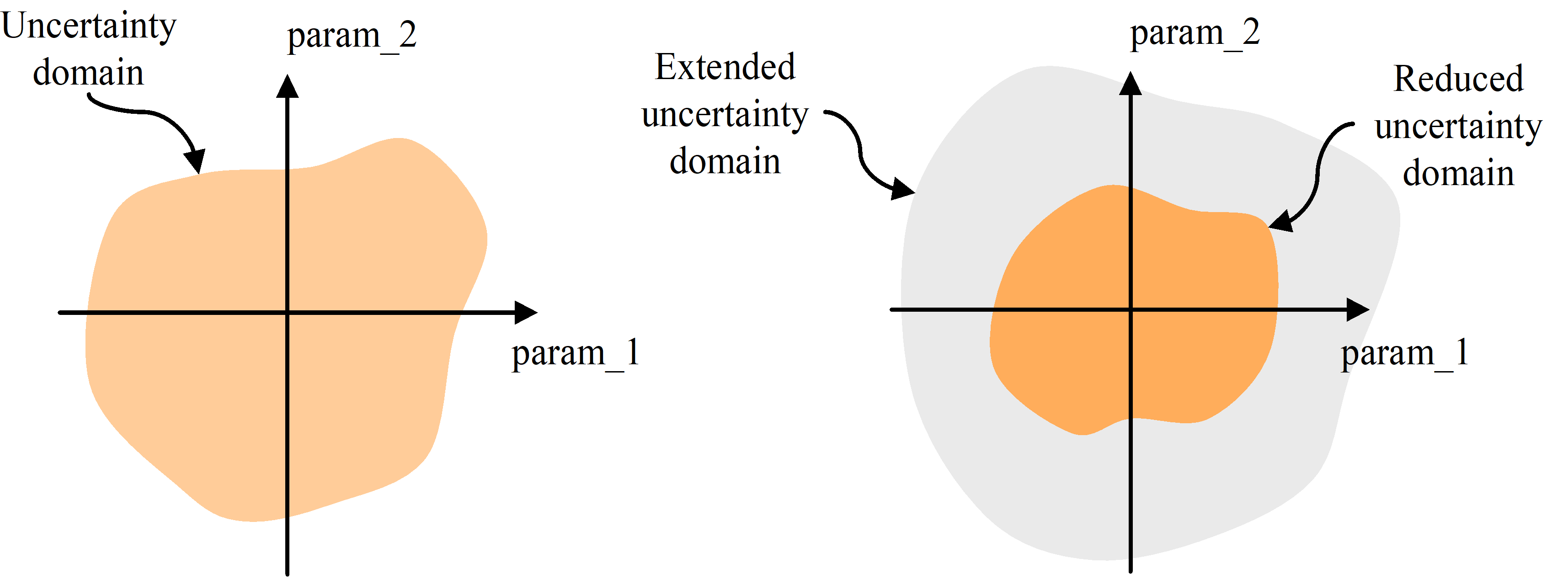Figure 51: Defining the uncertainty domains

Specification of an uncertainty domain

An uncertainty domain shall be defined identifying the set of physical parameters of the system over which the stability property is going to be verified.
This domain shall consist of:

• A list of the physical parameters to be investigated.
• For each of these parameters, an interval of uncertainty (or a dispersion) around the nominal value.
• When relevant, the root cause for the uncertainty.
• 1    The most important parameters for usual AOCS applications are the rigid body inertia, the cantilever eigenfrequencies of the flexible modes (if any), the modal coupling factors, and the reduced damping factors.
• 2    Usually the uncertainty or dispersion intervals are defined giving a percentage (plus and minus) relative to the nominal value.
• 3    These intervals can also be defined referring to a statistical distribution property of the parameters, for instance as the 95 % probability ensemble.
• 4    In practice the uncertainty domain covers the uncertainties and the dispersions on the parameters. In the particular case of a common design for a range or a family of satellites with possibly different characteristics and tunings, it also covers the range of the different possible values for these parameters.
• 5    The most common root causes for such uncertainties are the lack of characterization of the system parameter (for example: solar array flexible mode characteristics assessed by analysis only), intrinsic errors of the system parameter measurement (for example: measurement error of dry mass), changes in the system parameter over the life of the system, and lack of characterization of a particular model of a known product type.

Reduced uncertainty domain

A reduced uncertainty domain should be defined, over which the system operates nominally.

• 1    In the present context “operate nominally” means “verify nominal stability margins”.
• 2    The definition of this reduced uncertainty domain by the customer is not mandatory, and depends on the project validation and verification philosophy.
• 3    For the practical use of this reduced uncertainty domain, see Clause 5.2.7.

Extended uncertainty domain

An extended uncertainty domain should be defined, over which the system operates safely, but with potentially degraded stability margins agreed with the customer.

• 1    The definition of this extended uncertainty domain by the customer is not mandatory, and depends on the project validation and verification philosophy.
• 2    For the practical use of this extended uncertainty domain, see Clause 5.2.7.

Stability requirement

The stability property shall be demonstrated over the whole uncertainty domain.
If the uncertainty domain is split into a reduced and an extended domain according to 5.2.1, then the stability property shall be demonstrated over the extended domain.
The technique (or techniques) used to demonstrate the stability shall be described and justified.

Several methods are available for this purpose. For example stability of a linear time-invariant system can be demonstrated by examining the eigenvalues of the closed loop state matrix.

The point of the uncertainty domain leading to worst case stability should be identified.
The corresponding stability condition shall be verified by detailed time simulation of the controlled system.

Identification of checkpoints

Checkpoints shall be identified according to the nature and the structure of the uncertainties affecting the control system.

• 1    These loop checkpoints correspond to the points where stability margin requirements are verified. They are associated to uncertainties that affect the behaviour of the system.
• 2    Locating these checkpoints and identifying the associated types of uncertainties are part of the control engineering expertise; this can be quite easy for simple control loops (SISO systems), and more difficult for complex loops (MIMO, nested systems). Guidelines and technical detail on how to proceed is out of the scope of this document.

Selection and justification of stability margin indicators

For SISO loops the gain margin, the phase margin and the modulus margin shall be used as default indicators.
For MIMO loops the sensitivity and complementary sensitivity functions shall be used as default indicators.
The appropriate stability margin indicators shall be identified and justified by the control designer according to the nature and structure of the uncertainties affecting the system.
If other indicators are selected by the supplier, this deviation shall be justified and the relationship with the default ones be established.

• 1    The classical and usual margin indicators for SISO LTI systems are the gain and phase margins. Nevertheless in some situations these indicators can be insufficient even for SISO loops, and are completed by the modulus margin.
• 2    Sensitivity and complementary sensitivity functions are also valuable margin indicators for SISO systems. Actually the modulus margin is directly connected to the -norm of the sensitivity function.
• 3    Additional indicators, such as the delay margin, can also provide valuable information, according to the nature of the system and the structure of its uncertainties.
• 4    Selecting the most appropriate margin indicators is part of the control engineering expertise. Guidelines and technical detail on how to proceed is out of the scope of this document.

Stability margins requirements

Nominal stability margins are given by specifying values , , , and such that the following relations shall be met:

• The gain margin is greater than

• The phase margin is greater than

• The modulus margin is greater than

• The peak sensitivity and complementary sensitivity functions is lower than . Degraded stability margins are given by a specifying values , , and such that the following relations shall be met:

• The gain margin is greater than

• The phase margin is greater than

• The modulus margin is greater than

• The peak sensitivity and complementary sensitivity functions is lower than .

• 1    By definition , , and .

• 2    The numerical values to be set for these required margins are left to the expertise of the customer; there is no general rule applicable here, although values 6 dB, 30°, 6 dB can be considered “classical”.

Verification of stability margins with a single uncertainty domain

The nominal stability margins requirements shall be demonstrated over the entire uncertainty domain.

• 1    This clause applies in the case where a single uncertainty domain is defined – refer to 5.2.1.
• 2    the term “nominal stability margins” is understood according to 5.2.5, clause a.

Verification of stability margins with reduced and extended uncertainty domains

The nominal stability margins specified by the customer shall be demonstrated over the reduced uncertainty domain.
The degraded stability margins specified by the customer shall be demonstrated over the extended uncertainty domain.

• 1    This clause applies in the case where a reduced and an extended uncertainty domains are defined. Refer to 5.2.1.
• 2    The terms “nominal” and “degraded stability margins are understood according to 5.2.5, clauses a. and b. respectively.
• 3    This formulation avoids the risk of ambiguity mentioned in Clause 5.1 by clearly stating over which uncertainty domain(s) the margins are verified. Here a reduced uncertainty domain is defined, where a nominal level of stability margins is specified; in the rest of the uncertainty domain, degraded margins are accepted.

ANNEX(informative) Use of performance error indices

Formulating error requirements

More about error indices

A performance error generally has a complicated behaviour over time. To quantify this behaviour, a small set of error indices are introduced, in order to capture a particular aspect of their variation over time, such as the average over some interval, the short term variation or the drift. These are defined in Clause 3.2 and are illustrated in Figure A-1 and Figure A-2.

Error indices are generally the most convenient way to deal with such time-varying errors, but in some cases it can be more appropriate to use other means of quantifying the error, for example by looking at the spectrum in the frequency domain.

For spacecraft pointing errors, the indices usually are specified in terms of the Euler angles  (between the target and actual payload frames) or  (between the actual and estimated payload frames). Sometimes it is more appropriate to use another quantity instead, such as a directional error, or a more complicated parameter such as the offset between an instantaneous pointing direction and a target path across the sky. Similar choices can be made for other control systems.

For high frequency jitter errors, it can be preferable to formulate the requirements in terms of constraints on the body rates rather than attitude. Rate error indices can be defined by replacing the Euler angles in the given definitions with the difference between real and desired body rates,  = real-target. This does not just apply to body rates: the indices can be applied to any time varying quantity, such as position.

It can also be necessary to define more error indices to place constraints on other types of error variation. For example, it can be necessary to place a requirement on how much the error can change in a 5 second interval, in which case an error index can be introduced on the quantity e = e(t) – e(t–5).

Figure: Example showing the APE, MPE and RPE error indices

Figure: Example showing the PDE and PRE error indices

Statistical interpretation of requirements

Any error is a function both of time, t, and of a set of parameters which define the error behaviour:  = (t,{A}). Depending on the exact scenario, {A} can include – for a given design of the control system – such things as the physical properties of the spacecraft, sensor biases, orbit, and so on: indeed any parameter whose value affects the error should be included in the set. Generally, a parameter A does not have a single known value, instead there is a range of possible values described by a probability distribution P(A).

It is useful to introduce the concept of the statistical ensemble, which is the set of all possible combinations of {A}, or equivalently the set of all possible (t). This is illustrated in Figure A-3 for a simple case in which .

Now suppose that we have a requirement that there is a 90 % probability that APE() < 1º. This requirement can be met in different ways: either for 90 % of the time for all members of the statistical ensemble (Figure A-4, left), or for 100 % of the time for 90 % of the ensemble (Figure A-4, right), or some intermediate case.

Which of these should apply depends upon the details of the mission and the payload. For example, if we are trying to make sure that during an observation at least 90 % of the light ends up in the payload field of view, then the first case applies (90 % of the time), while if we require continuous observation then the second (90 % of the ensemble) is more appropriate.

When giving a pointing requirement for an index I, make it clear what the probability is referring to. This is known as the statistical interpretation of the requirement. There are three commonly used statistical interpretations:

The ensemble interpretation: there is at least a probability PC that I is always less than Imax. (I.e. a fraction PC of the members of the statistical ensemble have I < Imax at all times)

The temporal interpretation: I is less than Imax for a fraction PC of the time (i.e. this holds for any member of the ensemble)

The mixed interpretation: for a random member of the ensemble at a random time, the probability of I being less than Imax is at least PC.

Other statistical interpretations are possible, such as that a requirement is met for 95 % of the time over 95 % of possible directions on the sky; the three interpretations above can be though of as extreme cases. It is important that it is always made clear which interpretation is used, as the statistics are very different for the different cases. This is illustrated in Figure A-5 for a simple case where  =A sin(t).

Note that the temporal interpretation is supposed to hold for any member of the ensemble. Since the ensemble potentially includes extreme cases, unlikely to occur in reality, in practice a “modified temporal interpretation” is used, where the ensemble is redefined to exclude such situations. (For example, configurations with one or more parameters outside the 3 limits can be excluded from the ensemble.)

Figure: Example of a statistical ensemble of errors.

In this case the parameters are the mean and amplitude of the variation and the ensemble is the set of all possible combinations of these parameters.

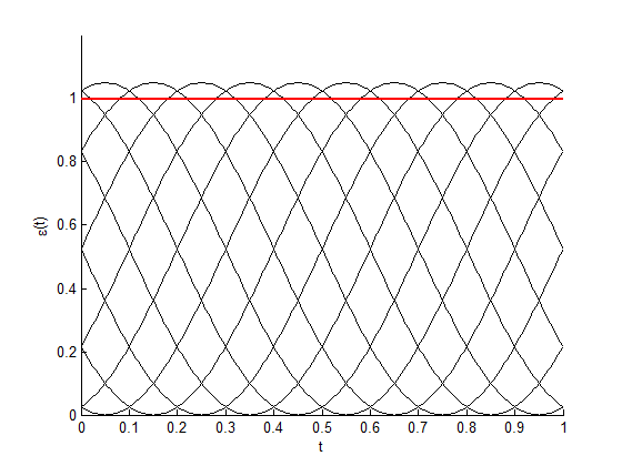
Figure: The different ways in which a requirement for P(||<1º) > 0,9 can be met

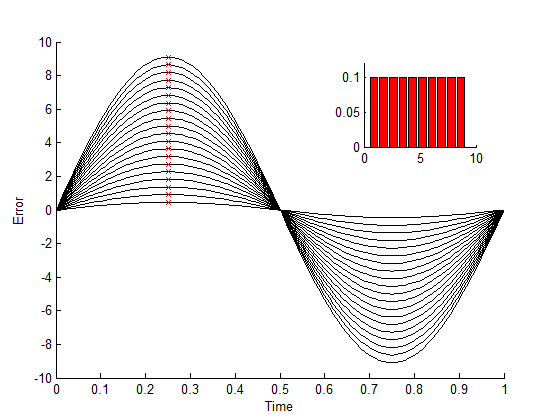
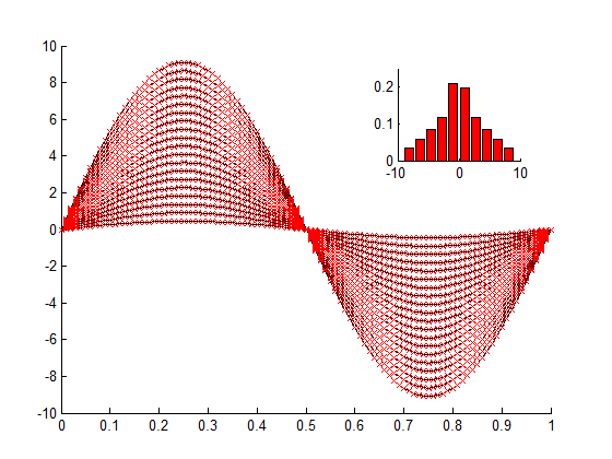Figure: Illustration of how the statistics of the pointing errors differ depending on which statistical interpretation is used

In this example  =A sin(t), where A has a uniform distribution in the range 0-10. Left: ensemble interpretation (worst case time for each ensemble member). Centre: temporal interpretation (all times for the worst case ensemble member). Right: Mixed interpretation (all times for all ensemble members).

Knowledge requirements

Knowledge requirements refer to the difference between the estimated state (sometimes known as the measured state, though this is misleading as the concept is more general than direct measurements) and the actual state.

When specifying knowledge requirements, the same considerations apply as for performance errors. The knowledge error indices defined in Clause 3.2 are used.

In addition, always make clear to what state of knowledge the requirement is referring to. For example, this can be

Direct outputs from a sensor

Knowledge available to the controller in (near) real time

Knowledge available for analysis after post-processing.

Specifying the timescales for requirements

The MPE, RPE, PDE and PRE indices defined in Clause 3.2, and their equivalents for knowledge errors, require one or more timescales for averaging (t, t1, t2) to be specified when giving a requirement. Usually, but not always, the same duration t is used for all of these indices.

Often there is an obvious choice for the averaging time, especially if there are discrete observations. For example: if the spacecraft is taking a succession of images, each lasting 1 minute, then all averaging should be done over a 1 minute observation period.

The MPE then represents the bias over an observation, the RPE the stability during the observation, and the PDE and PRE the difference between two observations which are nominally identical (see below). This discussion is in terms of the pointing of a spacecraft payload, but can be easily generalised to apply to other types of system.

In other cases this choice can be more complex, especially if continuous pointing is required over a long duration, with no natural breakdown into discrete periods. The averaging time t is specified some other way, for example by the minimum time required to collect useful data (payload integration time). However this time relates sensibly to the errors acting on the system: there is no point averaging over an integration time if all of the contributing errors have a longer period. In the end the choice comes down to a judgement of what is appropriate for the particular system.

For the PDE and PRE indices (drift and reproducibility), there is an additional timescale, namely the interval between the two averaging periods. Some ways in which such timescales can be defined are:

If the mission makes an extended observation, over many payload integration periods, then the duration of this observation should be used in the PDE definition.

If the mission is expected to keep its accumulated errors below some bounds for some minimum time (to avoid frequent calibrations requiring time out from normal mode), then this is the timescale which should be used in the PDE.

If there is a requirement that the mission should make an observation, and then be able to repeat this observation at some later time, then this timescale that should be used for the PRE definition.

It should be noted that the PDE and PRE indices are defined identically, except for whether or not there has been a calibration (resetting of accumulated errors) between the intervals.

It is also possible to define the PRE index without an explicit reference to a timescale, as the ability of the calibration process to return to an earlier state. In this type of situation, no quantitative value for the time interval TPRE is specified.

When specifying requirements it should always be made clear whether these timescales are treated statistically or as worst cases. Examples of how these can differ are:

PRE defined as a randomly chosen interval (in a continuous observation) and a randomly chosen time within that interval.

PRE defined as the worst case time within a randomly chosen interval.

PDE defined as difference between an observation at a random time and an observation a fixed period later.

PDE defined as the difference between an observation at local noon and an observation 12 hours later.

More about performance error budgets

When to use an error budget

Given a performance requirement for a spacecraft, the problem is to determine whether or not the design meets this requirement. There are various ways to check this:

Experimental results

Numerical simulations

A compiled error budget

Comparison with experimental results is not usually possible (at least for the complete system) until a late stage of development. Numerical simulations are more practical, but still have disadvantages. In particular, the only way to include ensemble type errors (see A.1.2) is to have some form of Monte-Carlo campaign with a large number of simulations covering the parameter space. Simulations are more useful for analysing specific contributions to the total pointing error (such as the controller behaviour) rather than the total pointing error for the entire system.

It is therefore usually necessary to compile an error budget for the system, to estimate the total error given what is known about the individual contributing errors. Ideally, a budget takes all known information about the contributing errors, use this to derive probability distribution functions (PDFs) for each one, and convolve these to find the PDF for the total error. This is impractical except in the very simplest cases: what is instead required is a simple rule to estimate the distribution of the total error so that is can be compared to the requirement.

It is important to be aware that such rules are approximations only, and that the assumptions made in the approximations can not always apply. The summation rules given in this standard are based on the central limit theorem, but this holds strictly true only in the limit N. However for a sufficiently large N the approximation is usually good enough. It is not always obvious what constitutes “sufficiently large”, but some rules of thumb can be applied:

If there are only a few contributing errors, or if one or two errors dominate over the others, then the approximation can be inappropriate, especially if one or more of these few errors have non-Gaussian form.

For example, if the budget is dominated by a sinusoidally varying error, then the probability distribution of the total error has a bimodal shape, not Gaussian.

As a rough guide, the APE and RPE indices generally have many contributors, while the PDE and PRE indices usually have only a few. (The MPE index can go either way depending upon the system.)

If the requirement is at a high confidence (e.g. 99,73 %) then small differences in the behaviour of the tails of the distribution changes whether the system is compliant or not.

In such cases more exact methods are recommended, though the approximate techniques used here are still useful for an initial rough assessment.

Identifying and quantifying the contributing errors

The first stage in compiling an error budget is to identify all the contributing error sources. These depend upon the system, so detailed guidelines cannot be given. As a general rule, follow a conservative approach, and include as many sources as possible rather than assuming that some are negligible; even small errors can contribute significantly if there are enough of them.

For pointing error budgets in particular, the different error sources often act in different frames, for example a sensor frame. Since the orientation affects how each error contributes to the error budget (see A.2.3) it is important to identify the right frame to use for each one.

Each individual error source has a probability distribution, which contributes to the statistics of the total error. Depending on which statistical interpretation is being applied, different probability distributions should be used:

For requirements of the ‘temporal’ type, use the statistics of the variation over time for the worst case ensemble member.

For requirements of the ‘ensemble’ type, use the statistics of the worst case values across the ensemble.

For requirements of the ‘mixed’ type, use the statistics across both time and the ensemble.

Figure A-5 illustrates the difference between these options. For most cases it is not necessary to obtain the full probability distribution, since to apply approximate methods only the means and variances are needed:

,        

How these quantities are obtained depend upon the error variation over time, the index being assessed, the statistical interpretation being applied, the available information regarding the ensemble parameters, and so on.

For many errors, such as sensor noise, the mean and variance of the error is supplied directly by the manufacturer.

For requirements using the ‘temporal’ statistical interpretation, there are generally simple formulae which can be applied, providing that the worst case ensemble parameters can be identified.

For requirements using the ‘ensemble’ statistical interpretation, the appropriate choice of PDF (and hence the formulae for mean and variance) depends upon how much is known about the ensemble parameter.

For requirements using the ‘mixed’ statistical interpretation, it is not trivial to find the means and variances of the overall distribution. However in many common cases approximate formulae exist.

More details can be found in Annex B together with formulae for some of the more common cases.

Combining the errors

Once the details of the contributing errors are known, the next step is to combine them to estimate the total error. This Clause gives combination methods, based on the central limit theorem, which are suitable in most cases. The approximation made is that the total form of the combined error is Gaussian, and as such is completely specified by its mean and standard deviation. However since this is an approximation it does not always apply. In particular, if the total error is dominated by a few highly non-Gaussian error sources then the approximations break down (see annex A.2.1.).

All individual errors do not contribute to the final result with the same weight, so determine the way they contribute before combining them. Taking the example of a spacecraft pointing budget, suppose that there are N independent errors contributing to the misalignment between payload and target frames. Each of these errors acts in a frame Fi (for i = 1 to N), such that the transformation between the nominal and real alignment of this frame is represented by error angles . The small angle approximation is assumed to apply, so that the order of the angles does not matter. The total error angle between the payload and target frames is then given by:

If we know the means {i,x, i,y, i,z} and standard deviations {i,x, i,y, i,z} for each individual contributing error (see Annex B) then the mean and variances of the total error angles are given by:

,

where is the total covariance matrix and are the individual covariance matrices, all square, of dimension (3,3). Considering the individual covariance matrices are diagonal gives a slightly simplified formula for the standard deviations:

Where means that each element of the matrix is squared individually, not the matrix as a whole. With the hypotheses considered, this is an exact expression for the mean and variance of a sum of contributing terms. Similar expressions can be derived for other systems in which the errors are linearly combined.

In the common case that all frames are nominally aligned, these expressions simplify:

,    

It is important to note that this approximation is based on the variance (²) of the individual contributing errors and not on their 68 % probability bound. Since we are making the approximation that the total distribution is Gaussian, this is now all the information required to define it completely.

These summation rules remain unaltered if, instead of taking the mean and variance directly, an error index is first applied:

,

That is, the error index applied to the total error is the sum of the error index applied to each of the contributing errors. This is the basis of the tables given in Annex B.

In the case where two errors are known or suspected to be correlated, it is recommended to alter slightly the summation rules for variance (to make them more conservative). Example are the cases in which two errors both vary at the orbital period, in which case it is very possible that they are both influenced by the same factors (phase of orbit, sun angle, etc.) and can therefore be in phase. Suppose that correlation is known (qualitatively) or suspected for two of the contributing errors (A and B). This can be dealt with by applying the more conservative approach of combining their standard deviations linearly instead of using the usual RSS formula:

The means are still summed linearly as before. The justification for this formula is that the two errors are effectively summed and treated as a single error (i.e. that the value of one depends upon the value of the other). It can however be more convenient to list them separately in a budget, to show that all effects have been included.

It is also possible to have a summation rule incorporating a factor expressing the degree of coupling, but since this involves determining the degree of coupling this is more complicated

Note that the summation rules given above are not the only ones that can be found in the literature. In particular, the approach adopted by the ESA pointing error handbook was to classify errors according to their time periods (short term, long term, systematic) and use a different way to sum between classes. This was an attempt to make the summation rules more conservative, and such rules have worked well in practice, but there is no mathematical justification for such approaches, and they can overestimate the overall variance if the inputs have been estimated well.

Comparison with requirements

Having estimated the distribution of the total error about each axis, this is compared to the requirement to see if the system is compliant.

In the case where the parameter being assessed in a linear sum of contributing errors (such as the Euler angles about each axis of a spacecraft) there is a simple formula; since the total distribution is assumed to have Gaussian form the system is compliant with the requirement providing that:

Where nP is defined such that for a Gaussian distribution the nP bound encloses a probability equal to the confidence level PC of the requirement. (The upper limit emax can be replaced by an upper limit on an error index, Imax).

To fix the ideas, let us remind that for a Gaussian distribution 1 is equivalent to PC = 68%, 2 is equivalent to PC = 95%, 3 is equivalent to PC = 99,7%.

The situation is more complicated if the total error is not a linear sum of contributors, as the final error does not have Gaussian distribution. The most common scenario for this is for directional errors of a payload boresight, for which the total error angle is found by taking the root sum square of the Euler angles about the perpendicular axes, for example:

.

The resulting distribution is not even close to having Gaussian shape. In the special case that both of the perpendicular axes have almost distributions with identical standard deviations total and negligible means, then the directional error follows a Rayleigh distribution, and the system is compliant to the requirement providing that:

Where, ‘log’ is the natural logarithm, base e.

For a requirement at 95 % confidence this translates into , while for 99,73 % confidence the condition is . Unfortunately if there is a significant mean, or if the standard deviations about the axes differ, then there is no such formula, however a simple numerical integration can be used instead, or a conservative estimate by taking both axes to be identical to the worst case one.

A simplified approach based on the approximation that the standard deviation of the error is the quadratic sum of the standard deviations of and leads to more conservative results. For example, with the hypothesis that both errors have negligible means and similar standard deviations, the requirement at 95% confidence gives , while for 99,73 % confidence the condition is

With directional errors, it is recommended to look very carefully at possible correlation between the two contributing axes. For example, if nutation causes the x-axis to rotate about its target direction at a constant offset angle, then the RPE of the directional error angle is zero, but both and have a significant RPE. Naively combining the two gives the wrong result for . In such cases, the correct thing to do is to look at the intention of the requirement (i.e. why is it important to constrain the RPE of ), and to be conservative in compiling the budget.

ANNEX(informative)Inputs to an error budget

Overview

The summation rules recommended in Clause 4.2.3 assume that the means and variances are known for all errors contributing to the total. In many cases these parameters can be easily available (quoted in a sensor specification for instance), in other cases it requires some work to obtain values, first deriving the probability distribution, then taking its mean and variance.

Some general rules should always be applied, the most important of which is to follow a conservative approach and to overestimate values rather than underestimate. As an example, assuming a-priori that a given error has an approximately Gaussian shape, identifying the bounds with the 3 (99,7 %) level and computing  and  accordingly, can in fact severely underestimate the value of σ if the error has a uniform distribution or sinusoidal form.

The values used differ depending upon the index being assessed (see Table B-1) and the statistical interpretation applied:

Ensemble interpretation: variation across the statistical ensemble at the worst case time. In this case, the mean and variance used in the budget refers to the variation of the possible worst case value, and depend upon the accuracy to which the ensemble parameters are known.

Temporal interpretation: variation over time for the worst case member of the statistical ensemble. In this case, the mean and variance used in the budget relates to the variation over time, and can be derived analytically if the time variation is known.

Mixed interpretation: variation across both time and over the statistical ensemble. It can be shown (see B.7) that in this case the correct value of the variance to use in the budgets is related to the root mean square (RMS) value of the ensemble parameter.

This Clause discusses the most common types of error, and gives tables to show the correct inputs to the budgets for different cases. Not all of the formulae given are exact, but they are generally a sufficiently good approximation. Other types of error can be analysed using similar methods.

In the tables of Annex B, the notations are as follows: E for “ensemble”, T for “time”, M for “mixed”; P(e) is the probability density function, (e) is the mean, and (e) is the standard deviation of the error.

Table: Parameters whose distributions are assessed for the different pointing error indices (knowledge error indices are similar)

Index being assessed	Parameter whose distribution is assessed	Description
APE		Error value over time
MPE		Mean error over a time interval
RPE	 , where 	Variation away from the mean
PDE	 , where Δt1, Δt2 are in same observation period	Change in the mean during an observation period
PRE	 , where Δt1, Δt2 are in different observation periods	Change in the mean between observation periods

Bias errors

A bias error is constant by definition, but this does not necessarily mean that its value cannot change during a mission. It is also possible to have a bias which is constant during an observation, but which changes between two different observations. For example, an attitude dependent star sensor error is constant so long as the sensor sees the same area of sky, but varies if its orientation changes.

This means that it is possible for bias errors to contribute to PRE index, providing that the bias changes between observations. Whether this is true, is assessed for each error separately.

Table B-2 shows the appropriate means and distributions for use with a bias error B. See B.6 for discussion of how to find distributions of the ensemble parameter B.

Table: Budget contributions from bias errors, where B represents the bias

Index	S.I.	Distribution			Index
		P(e)	μ(e)	σ(e)
APE	E	P(B)	μ B	 B	For P(B),  B and  B see B.6
	T	(BWC)	BWC	0	BWC=worst-case bias.
	M	P(B)	 B	 B	For P(B),  B and  B see B.6
MPE	All	As for APE			MPE
RPE	All	 (0)	0	0	No contribution by definition
PDE	All	 (0)	0	0	No contribution by definition
PRE	E	P(B)	0	2½  B	Only if bias can vary between observations, otherwise zero contribution.
	T	 (Bmax-Bmin)	Bmax-Bmin	0
	M	P(B)	0	2½  B

Random errors

Generally a random error has a Gaussian or quasi-Gaussian distribution, although there are cases (such as rounding errors or movement between bounds) for which a uniform distribution is appropriate. Random errors generally have a short period, and their distribution is assumed not to change significantly over time.

Often random errors come from sensors or actuators, in which case data are usually available directly from the suppliers’ specifications. If not, Table B-3 shows how to find the means and variances for Gaussian errors. In this case the ensemble parameter is the standard deviation (denoted ) itself: if this is not known but estimated then we are dealing with the standard deviation of the standard deviation, which is mathematically well defined (see B.6) but sounds confusing.

Also note that since Gaussian distributions do not have an upper bound, when looking at the ensemble distribution (worst case time) it becomes necessary to impose one. Using the 3 bound as a worst case is generally adequate.

Table B-4 gives the same information for uniform random errors with a range 0 to C, with C being the ensemble parameter in this case.

Table: Budget contributions from zero mean Gaussian random errors

Index	S.I.	Distribution			Notes
		P(e)	(e)	(e)
APE	E		3 	3	See text. For P(s),  and s see B.6
	T	G(0 , sWC2)	0	sWC	G(m,V) = Gaussian with specified mean & variance, sWC = worst case s
	M		0		For P(s), s and <s> see B.6. For derivation see B.7
MPE	All	0	0	0	Zero mean so no MPE contribution
RPE	All	As for APE			Zero mean so RPE identical to APE
PDE	All	No contribution			Short timescale, and assume mean value does not change over time
PRE	All
NOTE:    Zero mean is assumed; if a non-zero mean is present it can be treated as a separate bias-type error

Table: Uniform Random Errors (range 0-C)

Index	S.I.	Distribution			Notes
		P(e)	(e)	(e)
APE	E	P(C)	C	C	For P(C), C and C see B.6.
	T	U(0,CWC)			U(xmin,xmax) = uniform in range xmin to xmax. CWC = worst case C
	M				For P(C), μC and <C> see B.6. For derivation see B.7
MPE	E				For P(C), C and C see B.6.
	T			0	CWC = worst case C
	M				For P(C), C and <C> see B.6. For derivation see B.7
RPE	E				For P(C), C and C see B.6.
	T		0		U(xmin,xmax) = uniform in range xmin to xmax. CWC = worst case C
	M		0		For P(C), C and <C> see B.6. For derivation see B.7
PDE	All	No contribution			Short timescale, and assume mean value does not change over time
PRE	All

Periodic errors (short period)

By short period, it is meant that the timescale of variation is much shorter than the averaging time used in the indices, so that the average of the error is zero (any non-zero average can be treated as a separate bias-type error). The distribution of the error can be found assuming that it has sinusoidal form. Table B-5 shows the appropriate means and distributions to be used. See B.6 for discussion of how to find distributions of the ensemble parameter A (amplitude of the periodic error).

It is worth mentioning that there is a lot of literature dealing with the relationship between time and frequency domains requirements using the RPE, some of the relevant techniques being already in use in the industry. Refer for example to [1].

Table: Budget contributions for periodic errors (low period sinusoidal)

Index	S.I.	Distribution			Notes
		P(e)	(e)	(e)
APE	E	P(A)	A	A	For P(A), A and A see B.6
	T		0		AWC = worst case A
	M		0		For P(A), A and <A> see B.6 For derivation see B.7
MPE	All	0	0	0	No MPE for low period errors
RPE	All	As for APE			No mean so RPE, APE same
PDE	All	No contribution			No change over time so no contribution to PDE, PRE
PRE	All
NOTE:    Zero mean is assumed; if a non-zero mean is present it can be treated as a separate bias-type error

Periodic errors (long period)

By long period, it is meant that the timescale of variation is much longer than the averaging time used in the indices, so that to a good approximation the index does not change during an observation. The distribution of the error can be found assuming that it has sinusoidal form. Table B-6 shows the appropriate means and distributions to be used. See B.6 for discussion of how to find distributions of the ensemble parameter A.

Table: Budget contributions for periodic errors (long period sinusoidal)

Index	S.I.	Distribution			Notes
		P(e)	(e)	(e)
APE	E	P(A)	A	A	For P(A), A and A see B.6
	T		0		AWC = worst case A
	M		0		For P(A), A and <A> see B.6; For derivation see B.7
MPE	All	As for APE
RPE	All	0	0	0
PDE	E		2A	2A	Actual values depend on the definitions of PDE, PRE. These values are computed assuming a worst case where the 2 intervals are taken ½ period (time T/2) apart, so that e= 2e
	T		0	
	M		0	
PRE	All	As for PDE
NOTE:    Zero mean is assumed; if a non-zero mean is present it can be treated as a separate bias-type error

Distributions of ensemble parameters

In Clauses B.2 to B.5 the error statistics (in ensemble or mixed interpretations) depend on the statistics of the ensemble parameters A (periodic), B (bias), C (uniform random) and s (Gaussian random). For a general ensemble parameter, x, we need to be able to determine the probability distribution of x given the data available, in particular the mean and standard deviation.

Case 1: measured data. If a measurement is made of the parameter x, this gives a measured value plus some error range, xest ± x, where x corresponds to the n- level of a Gaussian. In this case the appropriate distribution is a Gaussian with:

    x = xest,    x = x /n

This is appropriate for example for the measured bias of a sensor.

Case 2: bounds known, distribution not known. If it is known that X is in the range xmin to xmax, and that intermediate values are possible, but no other information is available, then the appropriate distribution is a uniform distribution between these bounds. This is appropriate for example for alignment using shimming.

Case 3: PDF of ensemble parameter known. In such case the relevant properties can be extracted directly from the probability distribution:

Equation ,

Equation ,

This can occur if the physical process underlying the ensemble is known well enough to predict its behaviour. An example is a pointing error caused by position uncertainty, in which the distribution of the ensemble parameter can be obtained knowing the uncertainties in the process of determining the orbit.

Table B-7 gives some common distributions used to describe ensemble parameters, and their important properties.

Table: Some common distributions of ensemble parameters and their properties

Name	DistributionP(x)	Meanx	Variancex2	RMS<x>
Delta				 
Gaussian				 
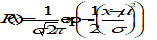
Uniform	 for  otherwise			
Bimodal (PDF for sinusoid)	 for  otherwise			

Using the mixed statistical distribution

When using the mixed statistical interpretation, there is a different temporal distribution (i.e. behaviour over time) for each value of the ensemble parameter. When taking the mean or variance, the appropriate PDF to quantify is the distribution over both time and ensemble:

Where normalisation constants are omitted.

However, rather than computing this distribution and then finding and , there is a simpler way. Starting from the definition of the mean

Substituting the above expression for P(x) and doing some manipulation gives

That is, the overall mean can be found using the distribution of A providing that the mean is known for a given value of A. Similarly for the variance 2:

This avoids computing the full distribution P(s). For example, suppose that we have a noise error with a zero mean Gaussian distribution over time:

In this case the ensemble parameter is the temporal standard deviation, S, and for a given value of S =0 and =S. If we know that S lies between 0 and Smax, but nothing else, then assuming a uniform distribution gives

Which is much easier than finding the full distribution

ANNEX(informative)Worked example

Scenario and requirements

Consider a simple scientific spacecraft, whose objective is to take images of various star fields, as shown in Figure C-1. Attitude measurement is done using a star sensor, attitude control using reaction wheels.

The requirements (formulated according to the recommendations of Clause 4.1) on the spacecraft are:

“The APE on the payload boresight shall be less than 20 arcsec about the y and z axes (the axes perpendicular to the boresight) and less than 1 arcmin about the x-axis (i.e. about the boresight)”.

“The RPE on the payload boresight shall be less than 10 arcsec about the y and z axes (the axes perpendicular to the boresight) and less than 30 arcsec about the x-axis (i.e. about the boresight), i.e. no more than half the error can be due sources which vary on short timescales. The timescale RPE is taken to be 30 seconds (the payload integration time)”.

“These requirements should be met for 95 % of the time using the ‘mixed’ statistical interpretation”

These requirements are derived from the payload parameters, such as field of view, pixel size, integration time and so on, as shown in Figure C-1. This derivation is beyond the scope of this note and so is not done here.

• 1    The example presented in this Annex is intended to illustrate the specification and budgeting procedure described in the standard, and does not intend to represent a real or even realistic spacecraft.
• 2    The performance budgets worked out in this Annex (clauses C.2 and C.3) are strictly based on the method described by Clause 4.2 (in particular the summation rules).
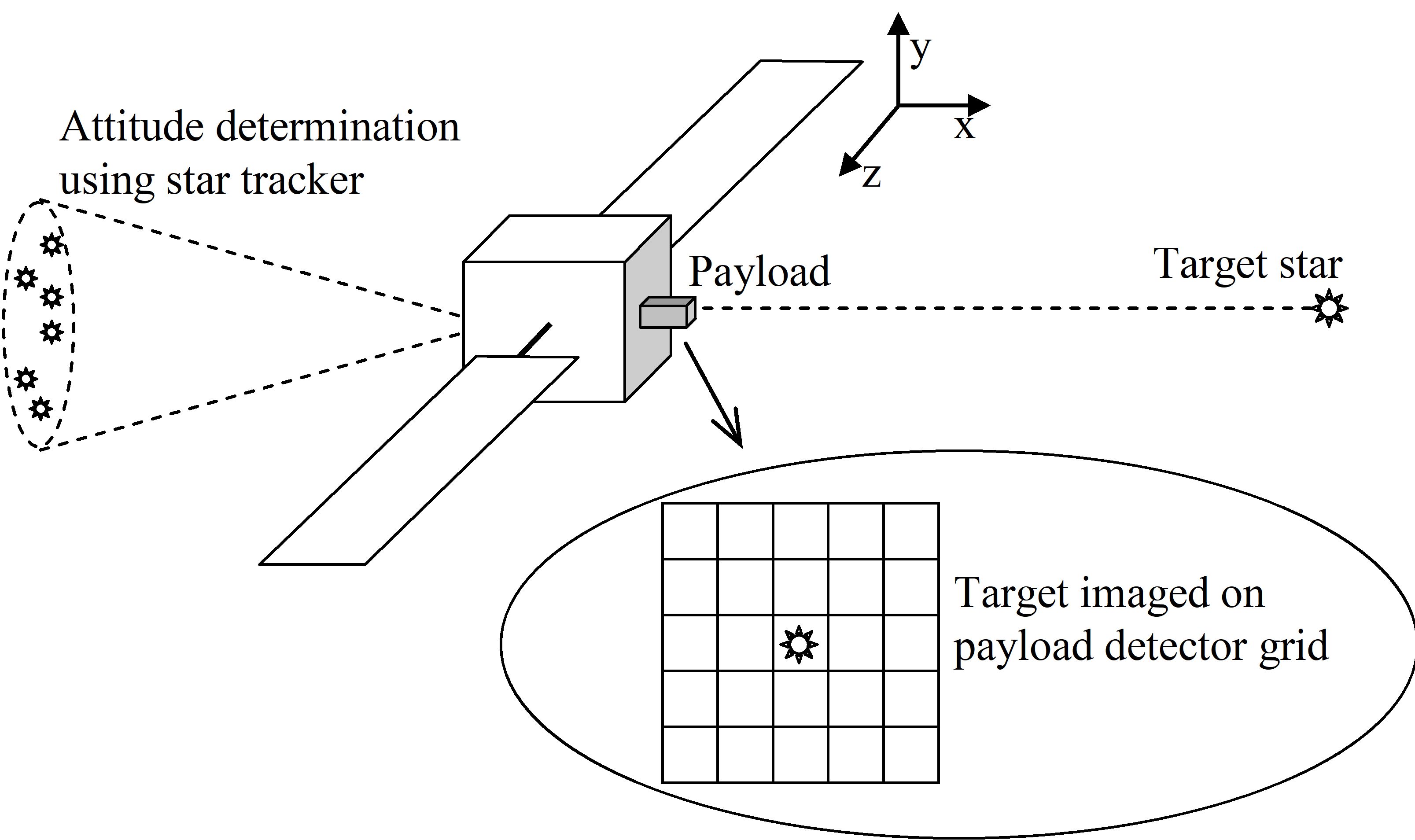  Figure: Scenario example

Assessing the contributing errors

For this example, the contributing errors can be classified into groups:

Measurement errors. The attitude measurement error of the star sensor is separated into two parts: an attitude dependent bias, and a time-dependent term. It is assumed that the distribution of the time varying errors (after filtering) is known exactly, but that of the attitude errors is not.

Control errors. The error in reaching the (measured) target frame. For the purpose of this example this also includes actuator errors (e.g. reaction wheel noise) as well as errors due to the controller itself. The resulting error distribution is assumed to be Gaussian, with a standard deviation (ensemble parameter) which is itself described by a Gaussian distribution.

Targeting errors. The dominant contribution here comes from the error in knowing the exact spacecraft position along its orbit, and hence the error varies sinusoidally at the orbital period.

Structural errors. The payload and the star sensor both have some misalignment with respect to the nominal body reference frame, so even after calibration there remains some misalignment between the two. In addition there is a thermoelastic distortion of the spacecraft, assumed to vary at the orbit period.

Table C-1 summarises these errors, together with their important properties. In order to provide some numerical inputs to the budget, the numerical values of the ensemble distribution are assumed to be those given in Table C-2. Note that these values are for illustration only, and are not necessarily representative of any given mission.

Note also that correlations between errors are not considered for this simple example.

Table: Example of contributing errors, and their relevant properties

Error	Temporal behaviour	Period	Ensemble distribution
STR time-dependent errors (after filtering)	Random	Less than observation period	Delta function (value known)
STR attitude dependent bias	Bias	observation period	Gaussian (variance known)
Controller and actuator errors	Random	Less than observation period	Gaussian (variance known)
Thermoelastic distortion STR & payload	Sinusoidal (assumed)	Orbit period	Uniform (range known)
Payload –STR misalignment after calibration	Bias	Does not vary	Uniform (range known)
Targeting error due to position knowledge	Sinusoidal	Orbit period	Gaussian (variance known)
Flexible modes & fuel slosh	Sinusoidal (assumed, not generally so simple)	Less than observation period	Gaussian (variance known)

The choice of the ensemble parameter distribution is different for each error:

The time dependent star sensor errors are assigned a delta-function distribution. This means that the value of the ensemble parameter (i.e. the noise level) are essentially known exactly

The thermoelastic distortion and payload/star sensor misalignment are assigned uniform distributions. This means that their bounds can be identified, but not the behaviour between them (see B.6)

The other errors are assigned Gaussian distributions, meaning that a distribution of their possible values is known. For example, the targeting error is related to the initial position error, and even though this is not known a-priori we can predict the probability of it having a particular value.

More details are given in Annex B.

Table: Example of distribution of the ensemble parameters

Error	Ensemble parameter E	dim	Distribution of ensemble parameter
			P(E)	E	E	<E>
STR time-dependent errors	Standard deviation over time	x	(10”)	10,0”	0	10,0”
		y	(5”)	5,0”	0	5,0”
		z	(5”)	5,0”	0	5,0”
STR attitude dependent bias	Value of bias	x	G(0, 6.67”)	0	6,67”	6,67”
		y	G(0, 3.33”)	0	3,33”	3,33”
		z	G(0, 3.33”)	0	3,33”	3,33”
Controller and actuator errors	Standard deviation over time	x	G(1”,3”)	1,00”	3,00”	3,16”
		y	G(1”,3”)	1,00”	3,00”	3,16”
		z	G(1”,3”)	1,00”	3,00”	3,16”
Thermoelastic distortion STR & payload	Amplitude of sinusoidal variation	x	U(0, 4”)	2,00”	1,15”	2,31”
		y	U(0, 4”)	2,00”	1,15”	2,31”
		z	U(0, 4”)	2,00”	1,15”	2,31”
Payload –STR misalignment	Value of bias	x	U(-5”,5”)	0	2,89”	2,89”
		y	U(-5”, 5”)	0	2,89”	2,89”
		z	U(-5”,5”)	0	2,89”	2,89”
Targeting error due to position knowledge	Amplitude of sinusoidal variation	x	G(0, 5”)	0	5,00”	5,00”
		y	G(0, 1”)	0	1,00”	1,00”
		z	G(0, 5”)	0	5,00”	5,00”
Flexible modes & fuel slosh	Amplitude of sinusoidal variation	x	G(0, 3”)	0	3,00”	3,00”
		y	G(0, 5”)	0	5,00”	5,00”
		z	G(0, 3”)	0	3,00”	3,00”
    (A) = delta function, G(,) = Gaussian distribution with specified mean and standard deviation, U(A,B) = uniform distribution with bounds A and B.

Compiling the pointing budgets

Using the values in Table C-2, the contributions to the pointing budgets for the APE and RPE indices can be worked out using the formulae given in annex B. Since the mixed statistical interpretation is being used here, all of the errors in the budget have zero mean, even if the ensemble parameter has non-zero mean. This is not the general case.

Combining the contributing standard deviations using the formula from Clause 4.2.3, it can be shown that the APE is compliant with the requirement (20 arcsec about y and 1 arcmin about x). However the RPE budget is not compliant with the requirement, as the short term variations are too large.

Table: Example of pointing budget for the APE index

Error	 (arcsec)			Formula from:
	x	y	z
STR time-dependent errors	10,0	5,0	5,0	Table B-3
STR attitude dependent bias	6,67	3,33	3,33	Table B-2
Controller and actuator errors	3,16	3,16	3,16	Table B-3
Thermoelastic: STR & payload	1,63	1,63	1,63	Table B-6
Payload –STR misalignment	2,89	2,89	2,89	Table B-2
Targeting error (position knowledge)	3,54	0,71	3,54	Table B-6
Flexible modes & fuel slosh	2,12	3,54	2,12	Table B-5
Total (RSS):	13,51	8,37	8,61	APE budget compliant
Total x 2 (for 95 % confidence):	27,01	16,75	17,21
Original requirement:	60	20	20

Table: Example of pointing budget for the RPE index

Error	 (arcsec)			Formula from:
	x	Y	z
STR time-dependent errors	10,0	5,0	5,0	Table B-3
STR attitude dependent bias	0,0	0,0	0,0	Table B-2
Controller and actuator errors	3,16	3,16	3,16	Table B-3
Thermoelastic: STR & payload	0,0	0,0	0,0	Table B-6
Payload –STR misalignment	0,0	0,0	0,0	Table B-2
Targeting error (position knowledge)	0,0	0,0	0,0	Table B-6
Flexible modes & fuel slosh	2,12	3,54	2,12	Table B-5
Total (RSS):	10,70	6,89	6,28	RPE budget not compliant
Total x 2 (for 95 % confidence):	21,40	13,78	12,57
Original requirement:	30	10	10

ANNEX(informative)Correspondence with the pointing error handbook

For the specific domain of AOCS and spacecraft pointing, the terminology introduced in this Standard brings in some innovation in regard to the ESA Pointing Error Handbook. This was made mandatory by the care for covering a more general field of application, not restricted to AOCS, and to deal with error signals of any physical type – not only angles and angular rates.

In order to help the user to switch to the new reference terms, Table D-1 explains how to translate the Pointing Error Handbook indicators into the ECSS- E-ST-60-10 ones:

Table: Correspondence between Pointing error handbook and ECSS-E-ST-60-10 indicators

PEH indicators	ECSS- E-ST-60-10 equivalence
APE (absolute pointing error)	APE (absolute performance error), applied to the pointing error
RPE (relative pointing error)	RPE (relative performance error), applied to the pointing error
PDE (pointing drift error)	PDE (performance drift error), applied to the pointing error
PRE (pointing reproducibility error)	PRE (performance reproducibility error), applied to the pointing error
MPE (median pointing error)	MPE (mean performance error), applied to the pointing error
AME (absolute measurement error)	AKE (absolute knowledge error), applied to the angular knowledge
ARE (absolute rate error)	APE (absolute performance error), applied to the angular rate
ARME (absolute rate measurement error)	AKE (absolute knowledge error), applied to the angular rate knowledge

.

References

“New definition of pointing stability: AC and DC effects” Lucke, Sirlin, San Martin. The Journal of the Astronautical Sciences Vol.40 No.4 Oct Dec 1992 pp 557-576.

Bibliography

ECSS-S-ST-00	ECSS system – Description, implementation and general requirements
ECSS-E-HB-60	Space engineering – Control engineering guidelines
ECSS-E-HB-60-10	Space engineering – Control performance guidelines