Space engineering

Stars sensors terminology and performance specification

Foreword

This Standard is one of the series of ECSS Standards intended to be applied together for the management, engineering and product assurance in space projects and applications. ECSS is a cooperative effort of the European Space Agency, national space agencies and European industry associations for the purpose of developing and maintaining common standards. Requirements in this Standard are defined in terms of what shall be accomplished, rather than in terms of how to organize and perform the necessary work. This allows existing organizational structures and methods to be applied where they are effective, and for the structures and methods to evolve as necessary without rewriting the standards.

This Standard has been prepared by the ECSS-E-ST-60-20 Working Group, reviewed by the ECSS Executive Secretariat and approved by the ECSS Technical Authority.

Disclaimer

ECSS does not provide any warranty whatsoever, whether expressed, implied, or statutory, including, but not limited to, any warranty of merchantability or fitness for a particular purpose or any warranty that the contents of the item are error-free. In no respect shall ECSS incur any liability for any damages, including, but not limited to, direct, indirect, special, or consequential damages arising out of, resulting from, or in any way connected to the use of this Standard, whether or not based upon warranty, business agreement, tort, or otherwise; whether or not injury was sustained by persons or property or otherwise; and whether or not loss was sustained from, or arose out of, the results of, the item, or any services that may be provided by ECSS.

Published by:     ESA Requirements and Standards Division
    ESTEC, ,
    2200 AG Noordwijk
    The
Copyright:     2008 © by the European Space Agency for the members of ECSS

Change log

ECSS-E-ST-60-20A	Never issued
ECSS-E-ST-60-20B	Never issued
ECSS-E-ST-60-20C 31 July 2008	First issue
ECSS-E-ST-60-20C Rev. 1 15 November 2008	First issue revision 1. Changes with respect to version C (31 July 2008) are identified with revision tracking. Main changes are: The term “imaginary ensemble” has been replaced in the whole document with “statistical ensemble” to be consistent with ECSS-E-ST-60-10.

Introduction

In recent years there have been rapid developments in star tracker technology, in particular with a great increase in sensor autonomy and capabilities. This Standard is intended to support the variety of star sensors either available or under development.

This Standard defines the terminology and specification definitions for the performance of star trackers (in particular, autonomous star trackers). It focuses on the specific issues involved in the specification of performances of star trackers and is intended to be used as a structured set of systematic provisions.

This Standard is not intended to replace textbook material on star tracker technology, and such material is intentionally avoided. The readers and users of this Standard are assumed to possess general knowledge of star tracker technology and its application to space missions.

This document defines and normalizes terms used in star sensor performance specifications, as well as some performance assessment conditions:

sensor components

sensor capabilities

sensor types

sensor reference frames

sensor metrics

Scope

This Standard specifies star tracker performances as part of a space project. The Standard covers all aspects of performances, including nomenclature, definitions, and performance metrics for the performance specification of star sensors.

The Standard focuses on performance specifications. Other specification types, for example mass and power, housekeeping data, TM/TC interface and data structures, are outside the scope of this Standard.

When viewed from the perspective of a specific project context, the requirements defined in this Standard should be tailored to match the genuine requirements of a particular profile and circumstances of a project.

This standard may be tailored for the specific characteristics and constraints of a space project in conformance with ECSS-S-ST-00.

Normative references

The following normative documents contain provisions which, through reference in this text, constitute provisions of this ECSS Standard. For dated references, subsequent amendments to, or revision of any of these publications, do not apply. However, parties to agreements based on this ECSS Standard are encouraged to investigate the possibility of applying the more recent editions of the normative documents indicated below. For undated references, the latest edition of the publication referred to applies.

ECSS-S-ST-00-01

ECSS system – Glossary of terms

Terms, definitions and abbreviated terms

Terms from other standards

For the purpose of this Standard, the terms and definitions from ECSS-S-ST-00-01 apply. Additional definitions are included in Annex B.

Terms specific to the present standard

Capabilities
aided tracking

capability to input information to the star sensor internal processing from an external source

1 This capability applies to star tracking, autonomous star tracking and autonomous attitude tracking.
2 E.g. AOCS.
angular rate measurement

capability to determine, the instantaneous sensor reference frame inertial angular rotational rates

Angular rate can be computed from successive star positions obtained from the detector or successive absolute attitude (derivation of successive attitude).

autonomous attitude determination

capability to determine the absolute orientation of a defined sensor reference frame with respect to a defined inertial reference frame and to do so without the use of any a priori or externally supplied attitude, angular rate or angular acceleration information

autonomous attitude tracking

capability to repeatedly re-assess and update the orientation of a sensor-defined reference frame with respect to an inertially defined reference frame for an extended period of time, using autonomously selected star images in the field of view, following the changing orientation of the sensor reference frame as it moves in space

1 The Autonomous Attitude Tracking makes use of a supplied a priori Attitude Quaternion, either provided by an external source (e.g. AOCS) or as the output of an Autonomous Attitude Determination (‘Lost-in-Space’ solution).
2 The autonomous attitude tracking functionality can also be achieved by the repeated use of the Autonomous Attitude Determination capability.
3 The Autonomous Attitude Tracking capability does not imply the solution of the ‘lost in space’ problem.
autonomous star tracking

capability to detect, locate, select and subsequently track star images within the sensor field of view for an extended period of time with no assistance external to the sensor

1 Furthermore, the autonomous star tracking capability is taken to include the ability to determine when a tracked image leaves the sensor field of view and select a replacement image to be tracked without any user intervention.
2 See also 3.2.1.9 (star tracking).
cartography

capability to scan the entire sensor field of view and to locate and output the position of each star image within that field of view

image download

capability to capture the signals from the detector over the entire detector Field of view, at one instant (i.e. within a single integration), and output all of that information to the user

See also 3.2.1.8 (partial image download).

partial image download

capability to capture the signals from the detector over the entire detector Field of view, at one instant (i.e. within a single integration), and output part of that information to the user

1 Partial image download is an image downloads (see 3.2.1.7) where only a part of the detector field of view can be output for any given specific ‘instant’.
2 Partial readout of the detector array (windowing) and output of the corresponding pixel signals also fulfil the functionality.
star tracking

capability to measure the location of selected star images on a detector, to output the co-ordinates of those star images with respect to a sensor defined reference frame and to repeatedly re-assess and update those co-ordinates for an extended period of time, following the motion of each image across the detector

sun survivability

capability to withstand direct sun illumination along the boresight axis for a certain period of time without permanent damage or subsequent performance degradation

This capability could be extended to flare capability considering the potential effect of the earth or the moon in the FOV.

Star sensor components
Overview

Figure 31 shows a scheme of the interface among the generalized componen specified in this Standard.

Used as a camera the sensor output can be located directly after the pre-processing block.

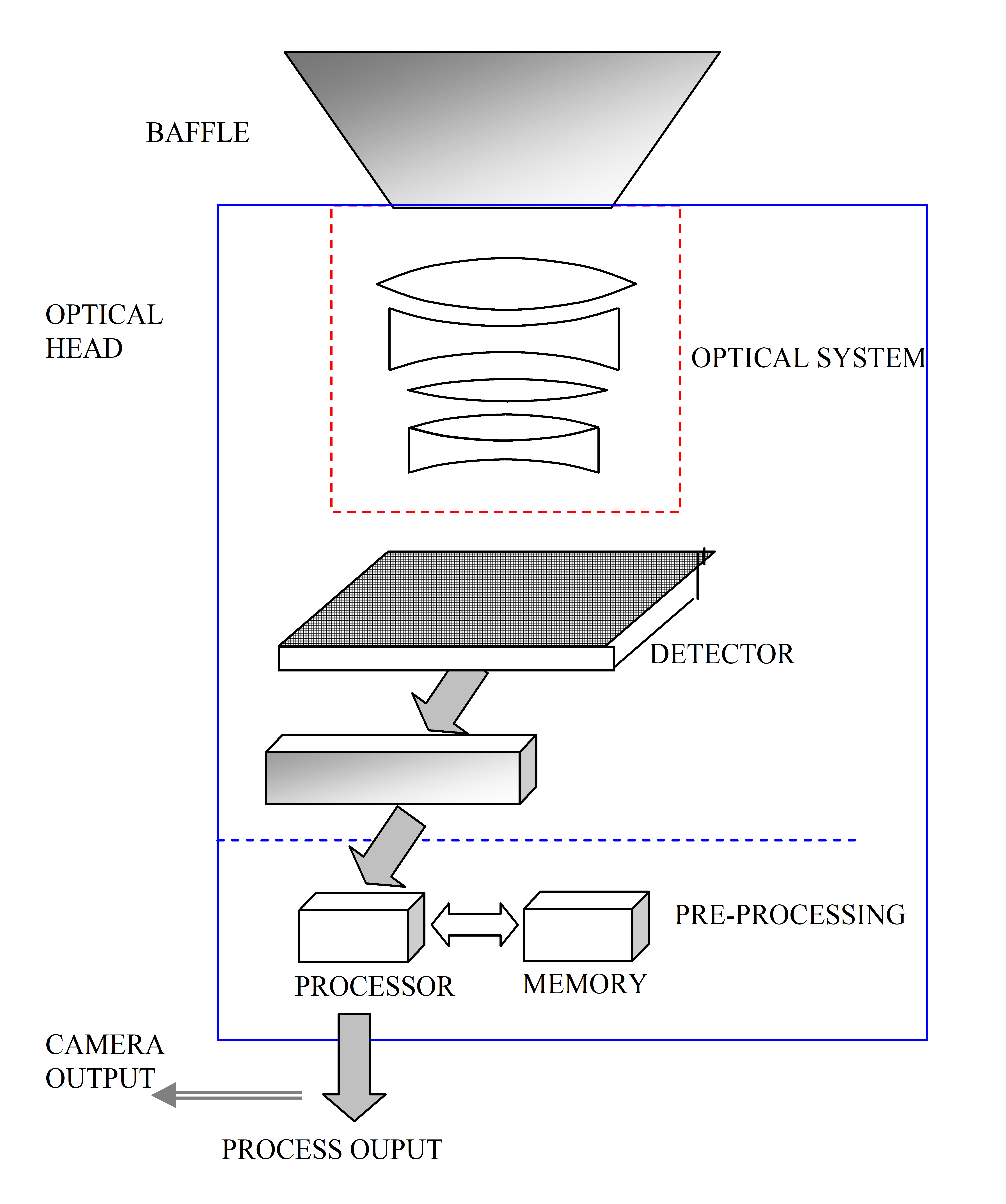Figure 31: Star sensor elements – schematic

baffle

passive structure used to prevent or reduce the entry into the sensor lens or aperture of any signals originating from outside of the field of view of the sensor

Baffle design is usually mission specific and usually determines the effective exclusion angles for the limb of the Earth, Moon and Sun. The Baffle can be mounted directly on the sensor or can be a totally separate element. In the latter case, a positioning specification with respect to the sensor is used.

detector

element of the star sensor that converts the incoming signal (photons) into an electrical signal

Usual technologies in use are CCD (charge coupled device) and APS (active pixel sensor) arrays though photomultipliers and various other technologies can also be used.

electronic processing unit

set of functions of the sensor not contained within the optical head

Specifically, the sensor electronics contains:

sensor processor;power conditioning;software algorithms;onboard star catalogue (if present).optical head

part of the sensor responsible for the capture and measurement of the incoming signal

As such it consists of

the optical system;the detector (including any cooling equipment);the proximity electronics (usually detector control, readout and interface, and optionally pixel pre-processing);the mechanical structure to support the above.optical system

system that comprises the component parts to capture and focus the incoming photons

Usually this consists of a number of lenses, or mirrors and filters, and the supporting mechanical structure, stops, pinholes and slits if used.

Reference frames
alignment reference frame (ARF)

reference frame fixed with respect to the sensor external optical cube where the origin of the ARF is defined unambiguously with reference to the sensor external optical cube

1 The X-, Y- and Z-axes of the ARF are a right-handed orthogonal set of axes which are defined unambiguously with respect to the normal of the faces of the external optical cube. Figure 32 schematically illustrates the definition of the ARF.
2 The ARF is the frame used to align the sensor during integration.
3 This definition does not attempt to prescribe a definition of the ARF, other than it is a frame fixed relative to the physical geometry of the sensor optical cube.
4 If the optical cube’s faces are not perfectly orthogonal, the X-axis can be defined as the projection of the normal of the X-face in the plane orthogonal to the Z-axis, and the Y-axis completes the RHS.
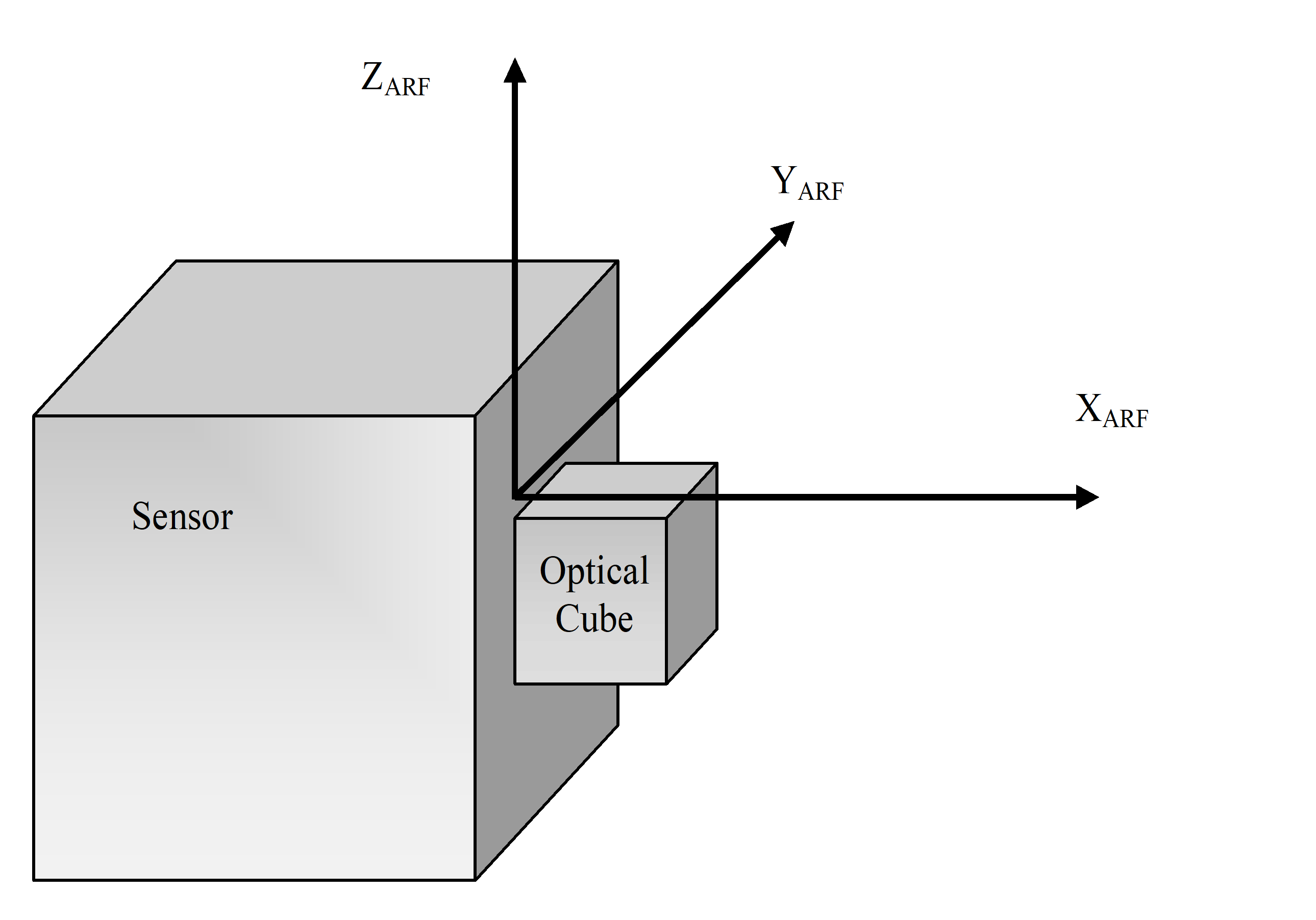Figure 32: Example alignment reference frame

boresight reference frame (BRF)

reference frame where:

the origin of the Boresight Reference Frame (BRF) is defined unambiguously with reference to the mounting interface plane of the sensor Optical Head;

In an ideally aligned opto-electrical system this results in a measured position at the centre of the detector.

the Z-axis of the BRF is defined to be anti-parallel to the direction of an incoming collimated light ray which is parallel to the optical axis;

X-BRF-axis is in the plane spanned by Z-BRF-axis and the vector from the detector centre pointing along the positively counted detector rows, as the axis perpendicular to Z-BRF-axis. The Y-BRF-axis completes the right handed orthogonal system.

1 The X-axes and Y-axes of the BRF are defined to lie (nominally) in the plane of the detector perpendicular to the Z-axis, so as to form a right handed set with one axis nominally along the detector array row and the other nominally along the detector array column. Figure 33 schematically illustrates the definition of the BRF.
2 The definition of the Boresight Reference Frame does not imply that it is fixed with respect to the Detector, but that it is fixed with respect to the combined detector and optical system.
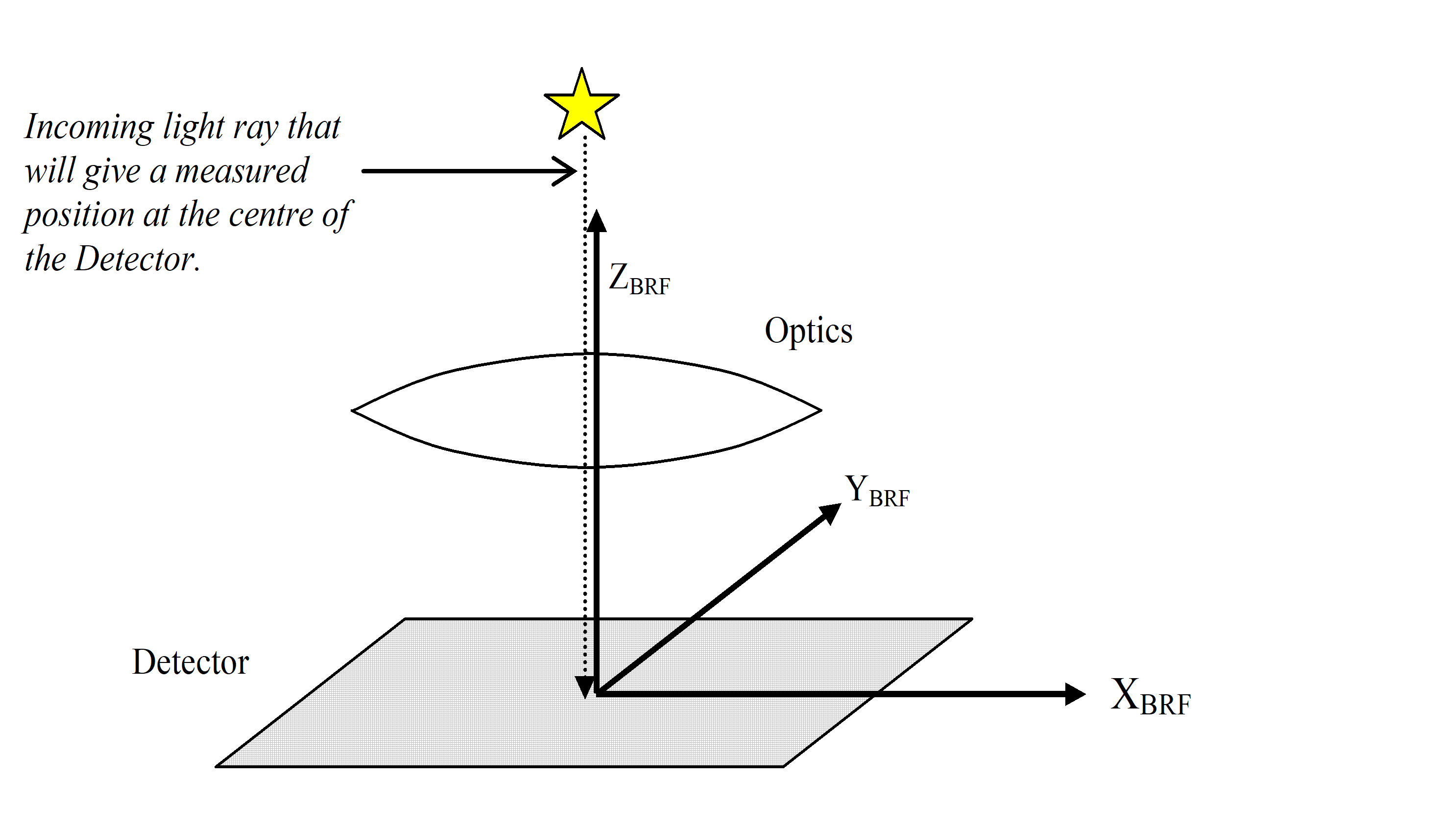Figure 33: Boresight reference frame

inertial reference frame (IRF)

reference frame determined to provide an inertial reference

1 E.g. use the J2000 reference frame as IRF as shown in Figure 34.
2 The J2000 reference frame (in short for ICRF – Inertial Celestial Reference Frame at J2000 Julian date) is usually defined as Z IRF = earth axis of rotation (direction of north) at J2000 (01/01/2000 at noon GMT), X IRF = direction of vernal equinox at J2000, Y IRF completes the right-handed orthonormal reference frame.
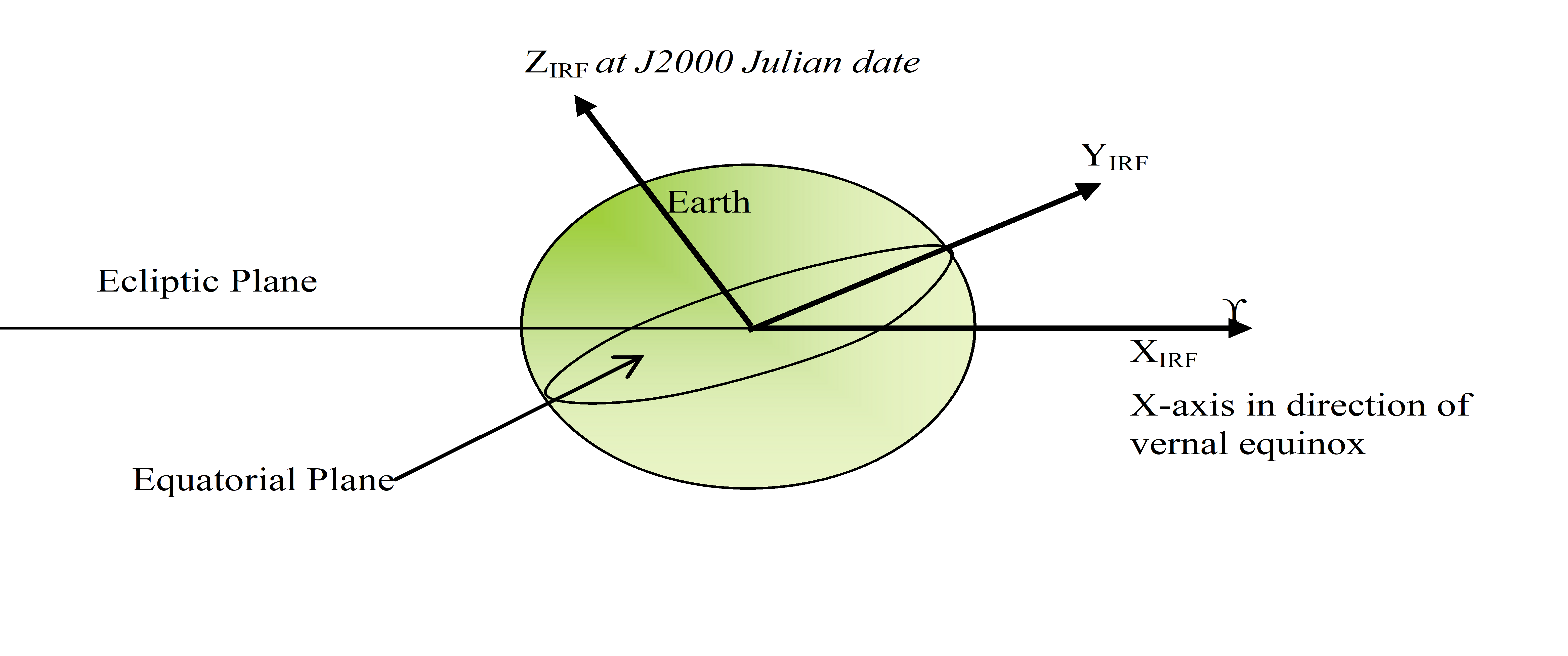Figure 34: Example of Inertial reference frame

mechanical reference frame (MRF)

reference frame where the origin of the MRF is defined unambiguously with reference to the mounting interface plane of the sensor Optical Head

1 For Fused Multiple Optical Head configurations, the interface plane of one of the Optical Heads may be nominated to define the MRF. The orientation is to be defined.
2 E.g. the Z-axis of the MRF is defined to be perpendicular to the mounting interface plane. The X- and Y-axes of the MRF are defined to lie in the mounting plane such as to form an orthogonal RHS with the MRF Z-axis.
3 Figure 35 schematically illustrates the definition of the MRF.
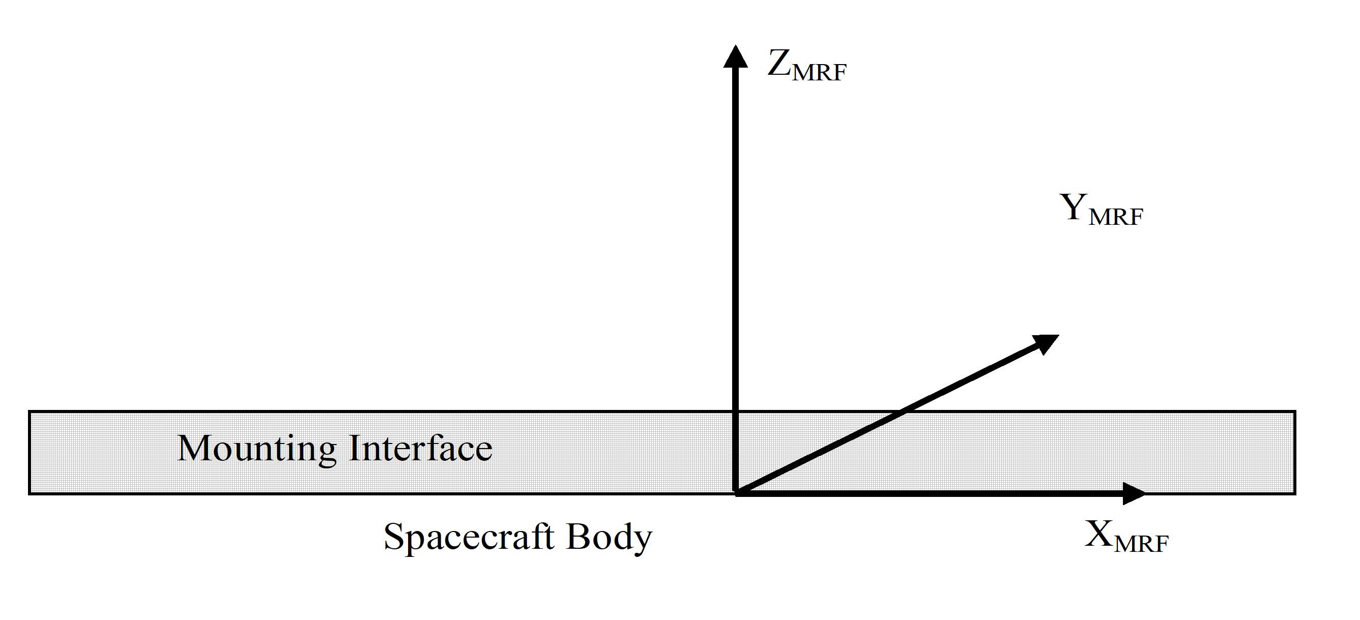Figure 35: Mechanical reference frame

stellar reference frame (SRF)

reference frame for each star where the origin of any SRF is defined to be coincident with the Boresight Reference Frame (BRF) origin

1 The Z-axis of any SRF is defined to be the direction from the SRF origin to the true position of the selected star Figure 36 gives a schematic representation of the reference frames. Figure 37 schematically illustrates the definition of the SRF.
2 The X- and Y- axes of the SRF are obtained under the assumption that the BRF can be brought into coincidence with the SRF by two rotations, the first around the BRF X-axis and the second around the new BRF Y-axis (which is coincident with the SRF Y-axis).
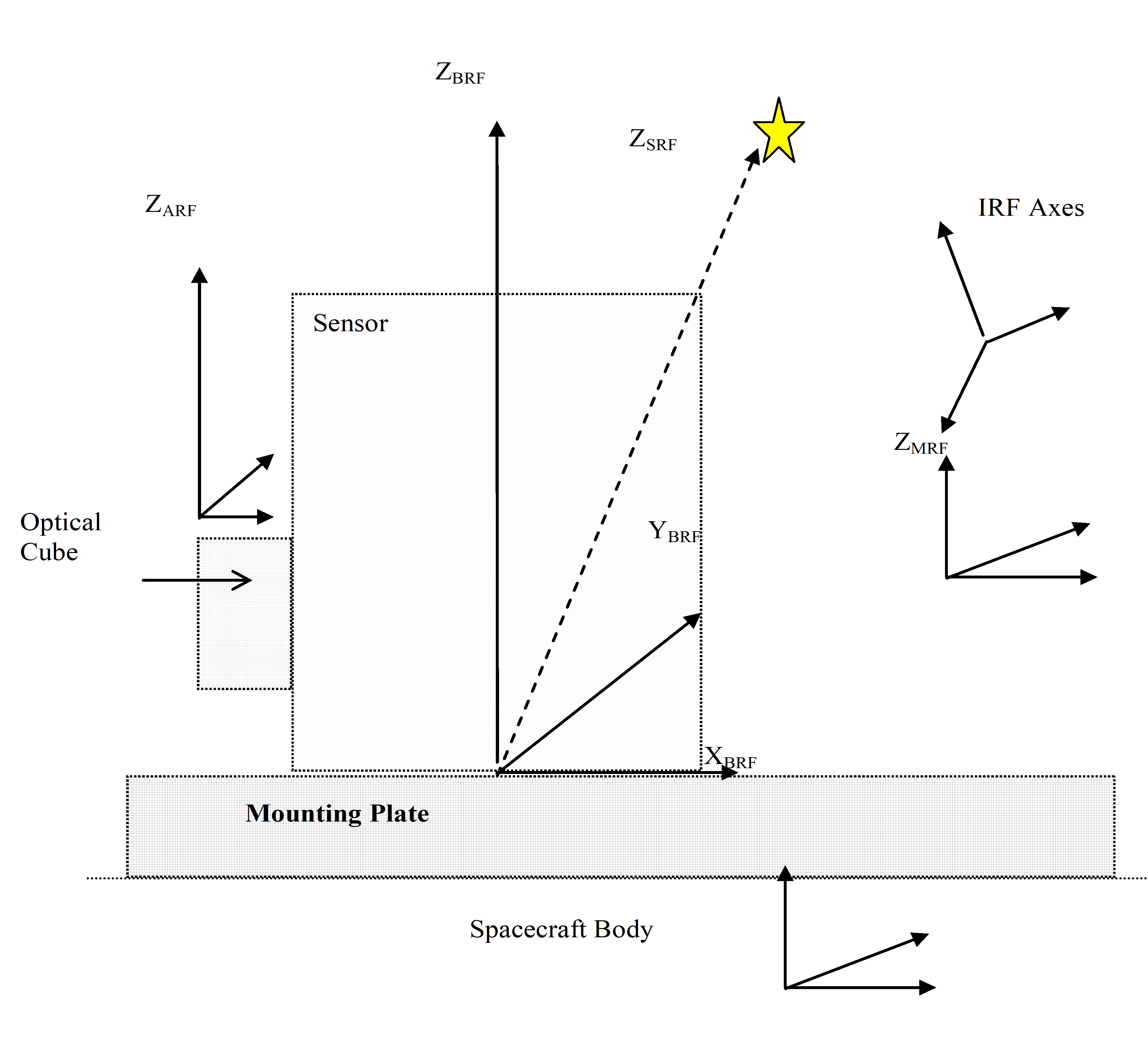Figure 36: Schematic illustration of reference frames

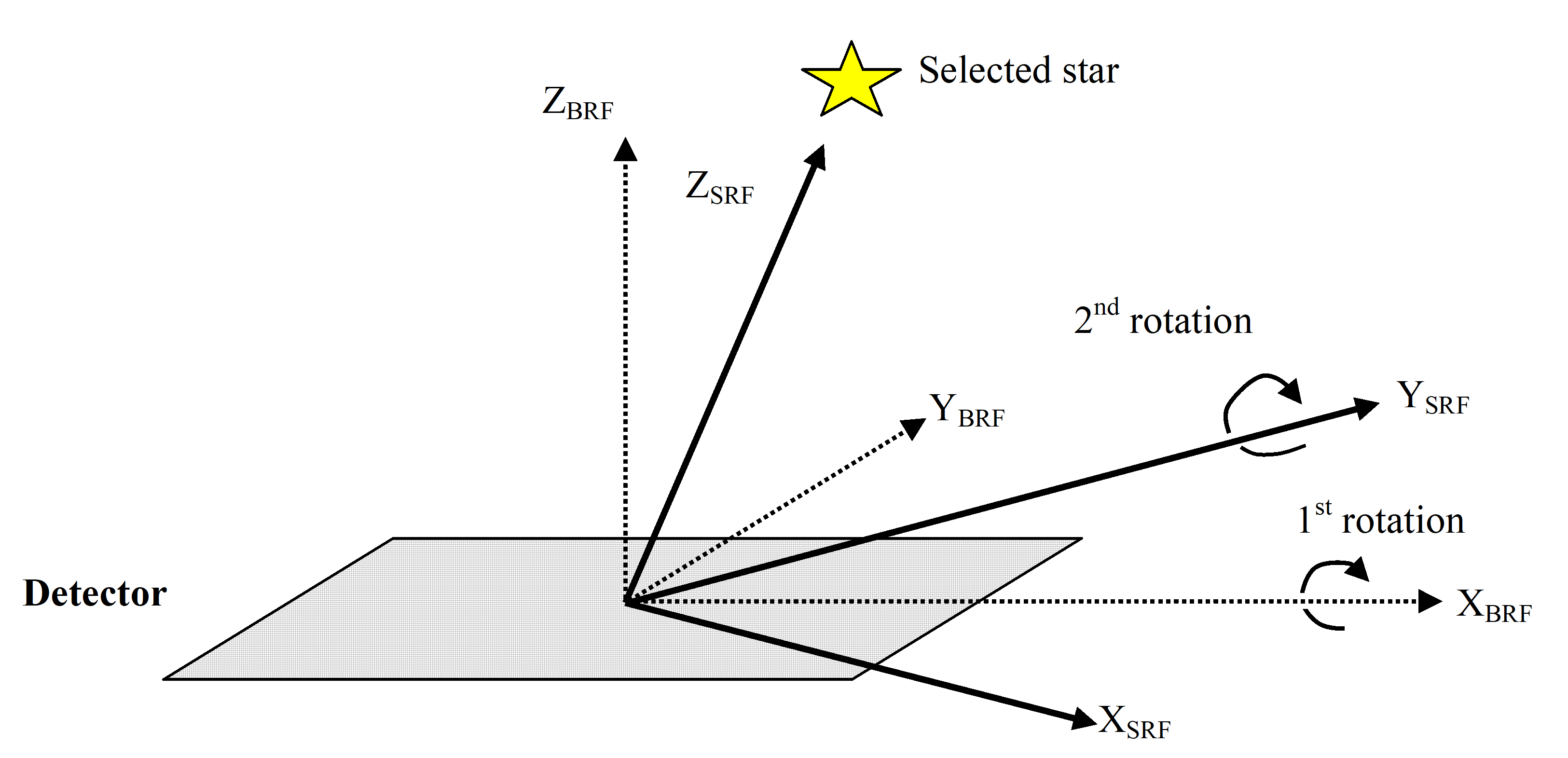Figure 37: Stellar reference frame

Definitions related to time and frequency
integration time

exposure time over which photons were collected in the detector array prior to readout and processing to generate the output (star positions or attitude)

1 Integration time can be fixed, manually adjustable or autonomously set.
2 Figure 38 illustrates schematically the various times defined together with their inter-relationship. The figure includes data being output from two Optical Heads, each of which is separately processed prior to generation of the sensor output. Note that for a Fused Multiple Optical Head sensor; conceptually it is assumed that the filtered output is achieved via sequential processing of data from a single head at a time as the data is received. Hence, with this understanding, the figure and the associated time definitions also ply to this sensor configuration.
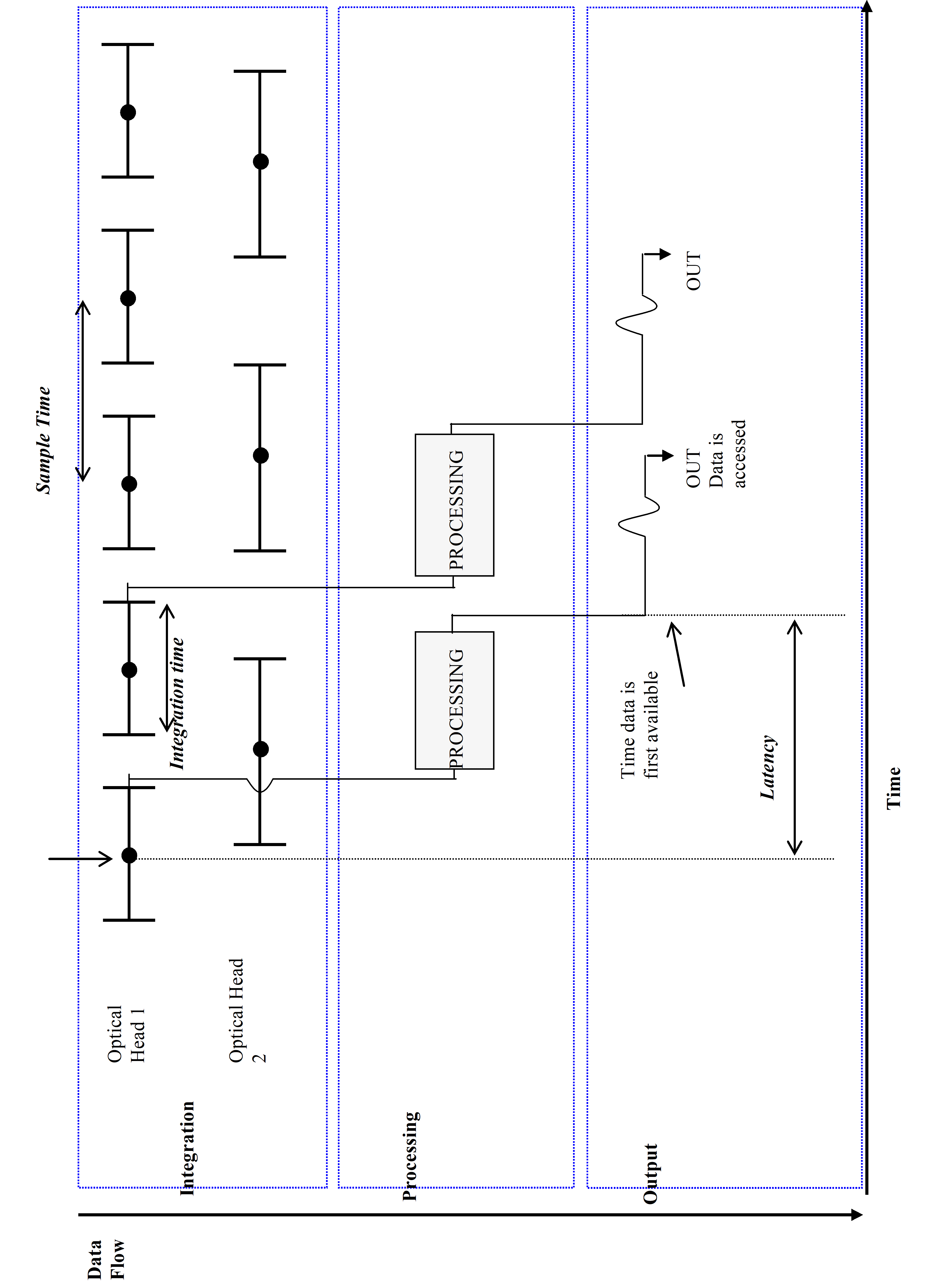Figure 38: Schematic timing diagram

measurement date

date of the provided measurement

1 In case of on board filtering the measurement date can deviate from individual measurement dates.
2 Usually the mid-point of the integration time is considered as measurement date for CCD technology.
output bandwidth

maximum frequency contained within the sensor outputs

1 The bandwidth of the sensor is limited in general by several factors, including:
integration time;sampling frequency;attitude processing rate;onboard filtering of data (in particular for multiple head units).* 2 The output bandwidth corresponds to the bandwidth of the sensor seen as a low-pass filter.
Field of view
half-rectangular field of view

angular region around the Boresight Reference Frame (BRF) frame Z-axis, specified by the angular excursions around the BRF X- and Y-axes between the BRF Z-axis and the appropriate rectangle edge, within which a star produces an image on the Detector array that is then used by the star sensor

1 This Field of View is determined by the optics and Detector design. This is schematically illustrated in Figure 39.
2 In the corners, the extent of the FOV for this definition exceeds the quoted value (see Figure 39).
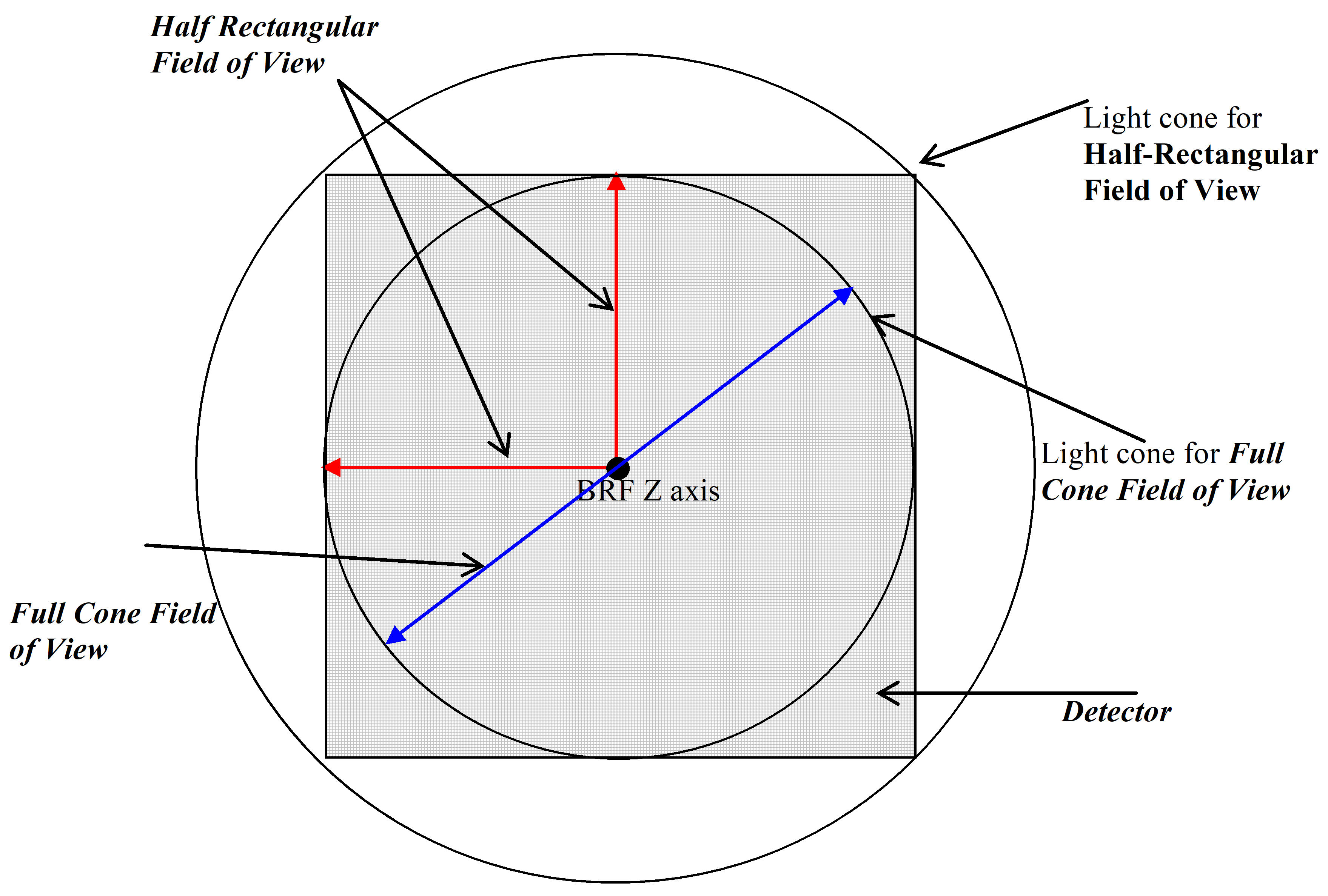Figure 39: Field of View

full cone field of view

angular region around the Boresight Reference Frame (BRF) frame Z-axis, specified as a full cone angle, within which a star will produce an image on the Detector array that is then used by the star sensor

This Field of View is determined by the optics and Detector design. This is schematically illustrated in Figure 39.

pixel field of view

angle subtended by a single Detector element

Pixel Field of View replaces (and is identical to) the commonly used term Instantaneous Field of View.

Angles of celestial bodies
aspect angle

half-cone angle between the Boresight Reference Frame (BRF) Z-axis and the nearest limb of a celestial body

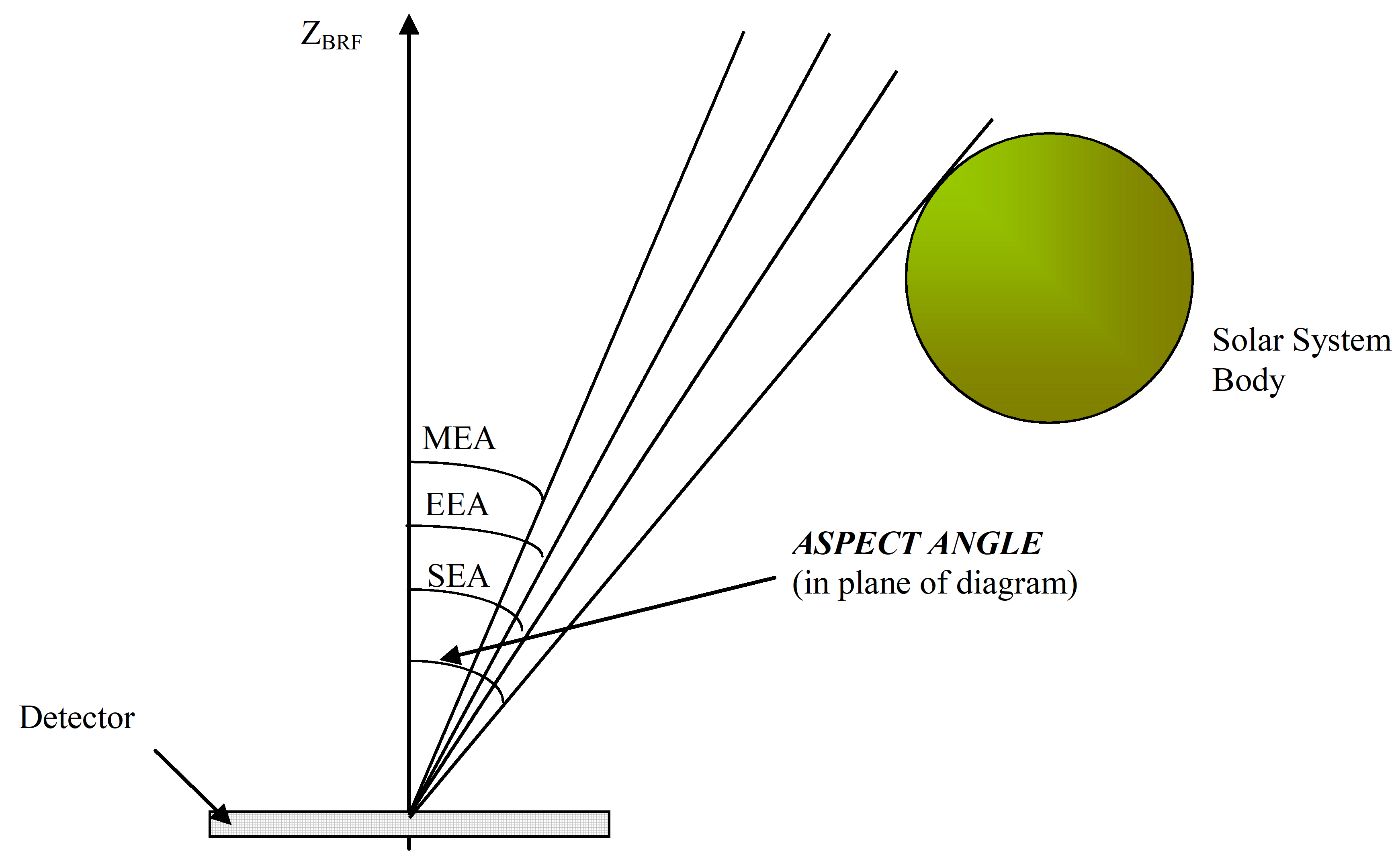Figure 310: Aspect angle to planetary body or sun

exclusion angle (EA)

lowest aspect angle of a body at which quoted full performance is achieved

1 The following particular exclusion angles can be considered:
The Earth exclusion angle (EEA), defined as the lowest aspect angle of fully illuminated Earth (including the Earth atmosphere) at which quoted full performance is achieved, as shown schematically in Figure 310.The Sun Exclusion Angle (SEA), defined as the lowest Aspect Angle of the Sun at which quoted full performance is achieved, as shown schematically in Figure 310.The Moon Exclusion Angle (MEA) is defined as the lowest Aspect Angle of the Full Moon at which quoted full performance is achieved, as shown schematically in Figure 310.* 2 The value of any EA depends on the distance to the object. In general, the bandwidth is the lowest of the cut-off frequencies implied by the above factors.
Most common terms
correct attitude

attitude for which the quaternion absolute measurement error (AMEq defined in D.2.2) is lower than a given threshold

correct attitude threshold

maximum quaternion absolute measurement error (AMEq) for which an attitude is a correct attitude

false attitude

attitude which is a non correct attitude

false star

signal on the detector not arising from a stellar source but otherwise indistinguishable from a star image

This definition explicitly excludes effects from the Moon, low incidence angle proton effects etc., which can generally be distinguished as non-stellar in origin by geometry.

image output time

time required to output the detector image

statistical ensemble

set of sensors (not all actually built) on which the performances are assessed by use of statistical tools on a set of observations and observation conditions

1 The statistical ensemble is defined on a case-by-case basis, depending on the performances to be assessed.
2 See 5.1 and Annex E for further details.
maintenance level of attitude tracking

total time within a longer defined interval that attitude tracking is maintained (i.e. without any attitude acquisition being performed) with a probability of 100 % for any initial pointing within the celestial sphere

This parameter can also be specified as Mean Time between loss of tracking or probability to loose tracking per time unit.

multiple star tracking maintenance level

total time within a longer defined interval that at least ‘n’ star tracks are maintained with a probability of 100 %

This covers the case where the stars in the FOV are changing, such that the star tracks maintained evolve with time.

night sky test

test performed during night time using the sky as physical stimulus for the star sensor. The effect of atmospheric extinction should be taken into account and reduced by appropriate choice of the location for test

probability of correct attitude determination

probability that a correct attitude solution is obtained and is flagged as valid, within a defined time from the start of attitude determination with the sensor switched on and at the operating temperature

1 Time periods for other conditions, like recovery after the Sun entering the FOV or a cold start, can be defined as the time needed to reach the start time of the attitude determination. The total time needed would then be the sum of the time needed to reach the start time of the attitude determination and the time period related to this metric.
2 Attitude solution flagged as valid means that the obtained attitude is considered by star sensor suitable for use by the AOCS. The validity is independent of accuracy.
3 Correct attitude solution means that stars used to derive the quaternion have been correctly identified, i.e. error on delivered measurement is below a defined threshold.
probability of false attitude determination

probability that not correct attitude solution is obtained, which is flagged as valid, within a defined time from the start of attitude determination with the sensor switched on and at the operating temperature

probability of invalid attitude solution

probability that an attitude solution (correct or not correct) is obtained and it is flagged as not valid, within a defined time from the start of attitude determination with the sensor switched on and at the operating temperature

1 The value of the Probability of Invalid Attitude Solution is 1-(Probability of Correct Attitude Determination + Probability of False Attitude Determination).
2 Invalid attitude solutions include cases of silence (i.e. no attitude is available from star sensor).
sensor settling time

time period from the first quaternion output to the first quaternion at full attitude accuracy, for random initial pointing within a defined region of the celestial sphere

The time period is specified with a probability of n% - if not quoted, a value of 99 % is assumed.

single star tracking maintenance probability

probability to be maintained by an existing star track over a defined time period while the tracked star is in the FOV

star image

pattern of light falling on the detector from a stellar source

star magnitude

magnitude of the stellar image as seen by the sensor

Star magnitude takes into account spectral considerations. This is also referred to as instrumental magnitude.

validity

characteristics of an output of the star sensor being accurate enough for the purpose it is intended for

E.g. use by the AOCS.

Errors
aberration of light

Error on the position of a measured star due to the time of propagation of light, and the linear motion of the STR in an inertial coordinate system

1 The Newtonian first order expression of the rotation error for one star direction is:
where:

V is the magnitude of the absolute linear velocity of the spacecraft w.r.t. to an inertial frame

c is the light velocity (299 792 458 m/s)

is the angle between the vector and the star direction

2 For a satellite on an orbit around the Earth, the absolute velocity is the vector sum of the relative velocity of the spacecraft w.r.t the Earth and of the velocity of the Earth w.r.t the Sun.
3 For an Earth orbit, the magnitude of this effect is around 25 arcsec (max). For an interplanetary spacecraft the absolute velocity is simply the absolute velocity w.r.t. the sun.
4 The associated metrics is the MDE (see Annex B.5.11 for the mathematical definition). The detailed contributors to the relativistic error are given in Annex G.
bias

error on the knowledge of the orientation of the BRF including:

the initial alignment measurement error between the Alignment Reference Frame (ARF) and the sensor Boresight Reference Frame (BRF) (on ground calibration)

the Alignment Stability Error (Calibration to Flight )witch is the change in the transformation between the sensor Mechanical Reference Frame (MRF) and the sensor Boresight Reference Frame (BRF) between the time of calibration and the start of the in-flight mission

1 The bias can be for the BRF Z-axis directional or the rotational errors around the BRF X, Y- axes.
2 For definition of directional and rotational errors see B.5.14 and B.5.17.
3 Due to its nature, the bias metric value is the same whatever the observation area is.
4 The associated metrics is the MME (see Annex B.5.7 for the mathematical definition). The detailed contributors to the bias are given in Annex G.
FOV spatial error

error on the measured attitude quaternion due to the individual spatial errors on the stars

1 This error has a spatial periodicity, whose amplitude is defined by the supplier. It ranges from a few pixels up to the full camera FOV.
2 FOV spatial errors are mainly due to optical distortion. These errors can be converted to time domain using sensor angular rate. Then, from temporal frequency point of view, they range from bias to high frequency errors depending on the motion of stars on the detector. They lead to bias error in the case of inertial pointing, while they contribute to random noise for high angular rate missions.
3 The associated metrics is the MDE (see Annex B.5.11 for the mathematical definition). The detailed contributors to the FOV spatial error are given in Annex G.
pixel spatial error

Measurement errors of star positions due to detector spatial non uniformities (including PRNU, DSNU, dark current spikes, FPN) and star centroid computation (also called interpolation error)

1 Because of their ‘spatial’ nature – these errors vary with the position of stars on the detector – they are well captured by metrics working in the angular domain. The pixel spatial errors are then well defined as the errors on the measured attitude (respectively the measured star positions) due to star measurement errors with spatial period of TBD angular value. Several classes of spatial periods can be considered.
2 These errors can be converted to time domain using sensor angular rate. Then, from temporal frequency point of view, they range from bias to high frequency errors depending on the motion of stars on the detector. They lead to bias error in the case of inertial pointing, while they contribute to random noise for high angular rate missions.
3 The associated metrics is the MDE (see Annex B.5.11 for the mathematical definition). The detailed contributors to the pixel spatial error are given in Annex G.
temporal noise

Temporal fluctuation on the measured quaternion (star positions) due to time variation error sources

1 Temporal noise is a white noise.
2 The associated metrics is the RME (see Annex B.5.8 for the mathematical definition). The detailed contributors to the temporal noise error are given in Annex G.
thermo elastic error

deviation of BRF versus MRF for a given temperature variation of the mechanical interface of the optical head of the sensor and thermal power exchange with space

1 The detailed contributors to the thermo elastic error are given in Annex G.
2 The associated metrics is the MDE (see Annex B.5.11 for the mathematical definition). FOV spatial error.
Star sensor configurations
fused multiple optical head configuration

more than one Optical Head, each with a Baffle, and a single Electronic Processing Unit producing a single set of outputs that uses data from all Optical Heads

independent multiple optical head configuration

more than one optical head, each with a baffle, and a single electronic processing unit producing independent outputs for each optical head

integrated single optical head configuration

single optical head plus baffle and a single electronic processing unit contained within the same mechanical structure

separated single optical head configuration

single optical head plus baffle and a single electronic processing unit which are not collocated within the same mechanical structure

Abbreviated terms

For the purpose of this Standard, the abbreviated terms from ECSS-S-ST-00-01 and the following apply:

Abbreviation	Meaning
AME	absolute measurement error
APS	active pixel sensor
ARF	alignment reference frame
ARME	absolute rate measurement error
AST	autonomous star tracker
BRF	boresight reference frame
BOL	beginning-of-life
CCD	charge coupled device
CTE	charge transfer efficiency
DSNU	dark signal non-uniformity
EEA	Earth exclusion angle
EOL	end-of-life
FMM	functional mathematical model
FOV	field of view
FPN	fix pattern noise
GRME	generalized relative measurement error
IRF	inertial reference frame
LOS	line of sight
MDE	measurement drift error
MEA	Moon exclusion angle
MME	mean measurement error
MRE	measurement reproducibility error
MRF	mechanical reference frame
PRNU	photo response non-uniformity
RME	relative measurement error
RHS	right handed system
SEA	Sun exclusion angle
SEU	singe event upset
SET	single event transient
SRF	stellar reference frame
STC	star camera
STM	star mapper
STR	star tracker
STS	star scanner

Functional requirements

Star sensor capabilities

Overview

This subclause describes the different main capabilities of star sensors. These capabilities are defined with respect to a generalized description of the reference frames (either sensor-referenced or inertially referenced in clause 3). This set of capabilities is then later used to describe the specific types of star sensor and their performances.

In order to describe the star sensor capabilities, the following generalized sensor model is used:

A star sensor comprises an imaging function, a detecting function and a data processing function. The imaging function collects photons from objects in the field of view of the sensor and focuses them on a detecting element. This element converts the photons into an electrical signal that is then subject to some processing to produce the sensor output.

A schematic of this sensor model is presented in Figure 41.

For each capability the nominal outputs and additional outputs are defined. These functional data should be identified in the telemetry list coming from the star sensor.

The outputs as defined in this document are purely related to the performance of the sensor, and represent the minimum information to be provided by the sensor to possess the capability. Other aspects, such as sensor housekeeping data, data structures and the TM/TC interface, are outside the scope of this Standard.

1 The same capabilities can be defined for Star Sensors employed on spinning spacecraft (Star Scanner) where star images are acquired at angular rate up to tens of deg/s driving the detector with a dedicated technique. For Star Sensor based on CCD detector, an example of this technique could be the Time Delay Integration (TDI). It is outside the scope of this specification to give detailed capability definitions for this kind of sensor.
2 Optional features are included in Annex B.6.
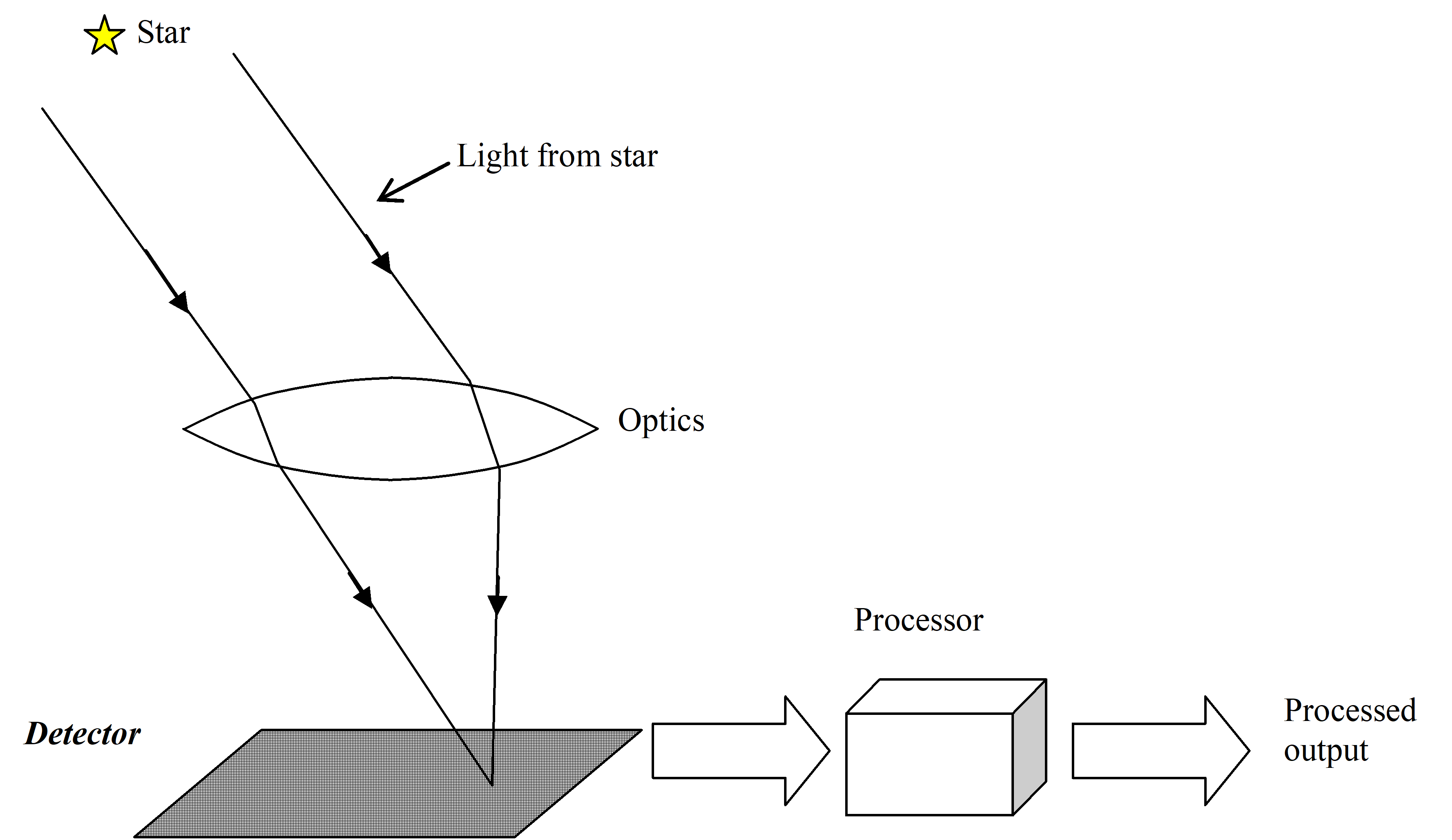Figure 41: Schematic generalized Star Sensor model

Cartography

Inputs

The acquisition command shall be supplied as minimum set of inputs.

Outputs

A sensor with cartography capability shall have the following minimum outputs:

star position,
measurement date. When the Star Image is measured in a Detector-fixed frame which is not the same as the Boresight Reference Frame (BRF), the output shall be converted into the Boresight Reference Frame (BRF).

The output parameterization is the Star Image position in the Boresight Reference Frame (BRF), given by the two measures of the angular rotations which define the transformation from the BRF to the star Stellar Reference Frame (SRF).

The date of measurement shall be expressed as a (scalar) number indicating the delay relative to a known external time reference agreed with the customer.

Star tracking

Inputs

The minimum set of inputs to be supplied in order to initialize the Star Tracking shall be:

the initial star position;
the angular rate;
validity date. For aided tracking, data specified in 4.1.3.1a shall be supplied regularly by the spacecraft, at an update rate and accuracy agreed by the customer.
The unit of all inputs shall be indicated.

Outputs

A sensor with the star tracking capability shall have the following minimum outputs:

the position of each Star Image with respect to a sensor-defined reference frame;
focal length if star position on the detector chip is output in units of length;
the measurement date.
1 The initial selection of the star images to be tracked by the sensor is not included within this capability and sometimes cannot be done without assistance external to the sensor.
2 The output parameterization is the Star Image position in the Boresight Reference Frame (BRF), given by the two measures of the angular rotations which define the transformation from the BRF to the star Stellar Reference Frame (SRF).
3 This capability does not imply to autonomously identify the star images as images to be tracked or explicitly identified by the unit. However, it does include the ability to maintain the identification of each star image and to correctly update the co-ordinates of each image as it moves across the detector due to the angular rate of the sensor.

Autonomous star tracking

Inputs

The minimum set of inputs to be supplied in order to initialize the Autonomous Star Tracking shall be:

the angular rate;
the validity date. For aided tracking, data specified in 4.1.4.1a shall be supplied regularly by the spacecraft, at an update rate and accuracy agreed by the customer.
The unit of all inputs shall be indicated.

Outputs

A sensor with the autonomous star tracking capability shall have the minimum outputs:

the position of each star image with respect to a sensor-defined reference frame;
the Measurement date.

This capability does not imply the stars to be explicitly identified by the unit. However, it does include the ability to maintain the identification of each star image once selected, to correctly update the co-ordinates of each image as it moves across the detector, and autonomously manage the set of star images being tracked.

Autonomous attitude determination

Inputs

The acquisition command shall be supplied as a minimum set of inputs.

When a priori initial attitude information for example an initial quaternion or a restriction within the celestial sphere, is supplied by the ground the capability is referred as Assisted Attitude determination

Outputs

A sensor with autonomous attitude determination shall have the minimum outputs:

the relative orientation of the defined sensor reference frame with respect to the defined inertial reference frame;

The relative orientation is usually expressed in the form of a normalized attitude quaternion

the Measurement date;
a validity index or flag estimating the validity of the determined attitude.

Autonomous attitude tracking

Inputs

The minimum set of inputs to be supplied in order to initialize the Autonomous Attitude Tracking shall be:

the attitude quaternion;
the 3-dimension angular rate vector giving the angular rate of the sensor BRF with respect to the IRF;

This vector is expressed in the sensor BRF.

the validity date for both supplied attitude and angular rate. For aided tracking, data specified in 4.1.6.1a shall be supplied regularly by the spacecraft, at an update rate and accuracy agreed by the customer.
Except for attitude quaternion, the unit of all inputs shall be indicated.
The supplier shall document whether the star sensor initialization uses either:
Internal initialization, or

The information to initialize the sensor is provided by the attitude determination function of the star sensor.

Direct initialization.

The information to initialize the sensor is supplied by an external source e.g. AOCS.

Outputs

A sensor with autonomous attitude tracking capability shall have the following minimum outputs:

the orientation of the sensor defined reference frame with respect to the inertially defined reference frame (nominally in the form of an attitude quaternion);
the Measurement date;
a validity index or flag, estimating the validity of the determined attitude;
measurement of Star Magnitude for each tracked Star Image.

Angular rate measurement

A sensor with angular rate measurement capability shall have the following minimum outputs:

the instantaneous angular rates around the Boresight Reference Frame (BRF) axes relative to inertial space;
the Measurement date. The date of measurement shall be expressed as a (scalar) number indicating the delay) relative to a known external time reference agreed with the customer.

The intended use of this capability is either when the attitude cannot be determined or to provide an angular rate.

(Partial) image download

Image download

A sensor with the (partial) image download capability shall have the following minimum outputs:

the signal value for each relevant detector element;
the Measurement date. Any use of image compression (e.g. for transmission) shall be documented.

The definition of the capability is intended to exclude ‘lossy’ image compression, though such compression can be a useful option under certain circumstances.

Image Output Time

The supplier shall specify the number of bits per pixel used to encode the detector image.
The image output time shall be verified by test using the hardware agreed between the customer and supplier.

1 The hardware used to perform the test is the hardware used to download the image from the star sensor.
2 For example:
“The Star Sensor shall be capable of performing a full Image Download of the entire Field of View at 12-bit resolution. The image output time shall be less than 10 seconds.”“The Star Sensor shall be capable of performing a partial Image Download at 12-bit resolution of a n×n section of the Field of View. The image output time shall be less than 10 seconds.”### Sun survivability

A sensor with the sun survivability capability shall withstand direct sun illumination along the bore sight axis, for at least a given period of time agreed with the customer, without subsequent permanent damage.
A sensor with the sun survivability capability shall recover its full quoted performances after the sun aspect angle has become greater than the sun exclusion angle.

Types of star sensors

Overview

This subclause specifies the nomenclature used to describe the different types of star sensors. Their classification is based on the minimum capabilities to be met by each type.

The term star sensor is used to refer generically to any sensor using star measurements to drive its output. It does not imply any particular capabilities.

The term Star Scanner is used to refer to a Star Sensor employed on spinning spacecraft. This kind of sensor performs star measurements at high angular rate (tens of deg/s). Formal capability definition of the Star Scanner, together with defined performance metrics are outside the scope of this specification.

Star camera

A star camera shall include cartography as a minimum capability.

Star tracker

A star tracker shall include the following minimum capabilities:

cartography;
star tracking.

If the autonomous star tracking capability is present, the cartography capability is internal to the unit when initializing the tracked stars and hence transparent to the ground.

Autonomous star tracker

An autonomous star tracker shall include the following minimum capabilities:

autonomous attitude determination (‘lost in space’ solution);
autonomous attitude tracking (with internal initialization). The supplier shall document whether the autonomous attitude determination capability is repetitively used to achieve the autonomous attitude tracking.

Reference frames

Overview

The standard reference frames are defined in 3.2.3.

Other intermediate reference frames are defined by the manufacturers in order to define specific error contributions, but are not defined here, as they are not used in the formulation of the performance metrics. See also Annex F.

Provisions

Any use of an IRF shall be accompanied by the definition of the IRF frame.
Any use of an attitude quaternion shall be accompanied by the definition of the attitude quaternion.

On-board star catalogue

The supplier shall state the process used to populate the on-board star catalogue and to validate it.
The process stated in 4.4a shall be detailed to a level agreed between the customer and the supplier.
The supplier and customer shall agree on the epoch at which the on-board star catalogue is valid.

In this context, ‘valid’ means that the accuracy of the on-board catalogue is best (e.g. the effect of proper motion and parallax is minimized).

The supplier shall state the epoch range over which performances are met with the on-board star catalogue.
The supplier shall deliver the on-board star catalogue, including the spectral responses of the optical chain and detector.
If the star sensor has the capability of autonomous attitude determination, the supplier shall deliver the on-board star pattern catalogue.
The maintenance process of the on-board star catalogue shall be agreed between the customer and the supplier.

1 The maintenance process includes the correction of parallax and the correction of the star proper motions in the on-board star catalogue.
2 The maintenance process includes the correction of the on-board catalogue errors identified in flight (e.g. magnitude, coordinates).
The supplier shall state any operational limitations in the unit performance caused by the on-board catalogue (e.g. autonomous attitude determination not possible for some regions in the sky). These limitations shall be agreed upon between the supplier and the customer.

Performance requirements

Use of the statistical ensemble

Overview

Performances have a statistical nature, because they vary with time and from one realization of a sensor to another. This clause presen the knowledge required to build performances up. Full details can be found in Annex E.

Only an envelope of the actual performances can be provided. Central to this is the concept of a ‘statistical ensemble’, made of ‘statistical’ sensors (i.e. not necessarily built, but representative of manufacturing process variations) and observations (depending on time and measurement conditions).

Three approaches (called statistical interpretations) can be taken to handle the statistical ensemble:

Temporal approach: performances are established with respect to time.

Ensemble approach: performances are established on statistical sensors (i.e. not necessarily built), at the worst case time.

Mixed approach, which combines both the approaches above.

The conditions elected to populate the statistical ensemble are defined on a case-by-case basis for each performance parameter, as described in the following clauses.

Provisions

The performances shall be assessed by using the worst-case sensor of the statistical ensemble.
The statistical ensemble shall be characterized and agreed with the customer.
The performances shall be assessed by using the sensor EOL conditions agreed with the customer.

The EOL conditions include e.g. aging effects, radiation dose.

Use of simulations in verification methods

Overview

Simulations efficiently support the verification of performances. A set of simulations provides an estimate of a performance, obtained by processing the simulation results in a statistical fashion. Because the set of simulations is limited, the performance estimated by simulations has a given accuracy, essentially depending on the number of simulations.

Provisions for single star performances

Software models of single star measurement error shall be validated for single star performance (at zero body rates) against on-ground tests using artificial stellar sources.

Denoting the confidence level to be verified as PC, and assuming that the performance confidence level result to be obtained is to an accuracy P with 95 % estimation confidence level, the number of Monte-Carlo runs to be performed is greater than .

Provisions for quaternion performances

Software models of attitude quaternion error shall be validated against on-ground tests using artificial stellar sources or with on ground tests agreed by the customer.

1 Denoting the confidence level to be verified as PC, and assuming that the confidence result to be obtained is to an accuracy P with 95 % confidence, the number of Monte-Carlo runs to be performed is greater than .
2 Refer to Annex E.1 for further details.

Confidence level

The following confidence level shall be agreed with the customer (see 5.5):

for the thermo elastic error;
for the FOV spatial error;
for the pixel spatial error;
for the temporal noise;
for the measurement date error;
Refer to Annex E for further details.
1 A performance confidence level of 95 % is equivalent to a 2 sigma confidence level for a Gaussian distribution.
2 A performance confidence level of 99,7 % used is equivalent to a 3 sigma confidence level for a Gaussian distribution.

General performance conditions

The performance conditions of the ‘statistical ensemble’ shall be used to encompass the following conditions for EOL:

worst-case baseplate temperature within specified range;
worst-case radiation flux within specified range;
worst-case stray light from solar, lunar, Earth, planetary or other sources.
1 In addition values for BOL can be given.
2 Worst-case stray light conditions are with the Sun, Earth and (where appropriate) Moon simultaneously at their exclusion angles together with worst-case conditions for any other light sources.
The maximum magnitude of body rate shall be used.

The maximum body rate is the worst case condition for most missions. For specific cases, the worst case can be adapted, e.g. to include jitter.

The supplier shall identify the worst case projection in BRF of the value defined in 5.4d.

Different angular rates can be specified with associated required performance.

The maximum magnitude of angular acceleration shall be used.

The maximum angular acceleration is the worst case condition for most missions. For specific cases, the worst case can be adapted, e.g. to include jitter.

The supplier shall identify the worst case projection in BRF of the value de-fined in bullet ‎d.

Different angular accelerations can be specified with associated required performance.

For multiple head configuration the worst case conditions of angular rate and stray light of each optical head shall be discussed and agreed between supplier and customer.
Single star position measurement performance within the verification simulations shall be:

validated against on-ground test data for fixed pointing conditions, and
able to predict metric performance under these conditions with an accuracy of 10 %. If test data is available for the individual error sources, the simulation shall be validated against this data with an accuracy of 10%.
Detector error sources in the simulation shall also be validated using direct data injection into the electronics and analysis of the test outpu.
The simulation allows the verification to cover the full range of conditions, including stray light, finite rates/accelerations, full range of instrument magnitudes, and the worst-case radiation exposure.
EOL simulations used to predict EOL performance shall be verified by test cases verifiable against measurable BOL data.
The impact of individual star errors on the overall rate accuracy shall be provided via simulation.
No aided tracking shall be considered.

General performance metrics

Overview

Clause 5.5 presen the general performance metrics for the error contributing to the star sensor performances. In Annex H, an example of data sheet built on the performance metrics is given.

Bias

General

The confidence level specified in clause 5.3 shall be used.
The ‘Ensemble’ interpretation shall be used as follows:

The Ensemble interpretation is as follows:

A statistical collection of sensors is arbitrarily chosen.A given set of observations is arbitrarily chosen.The specification for this type of variability is ‘less than the level S in confidence level n% of a statistical ensemble of sensors/observations for the worst-case time’.The bias performance shall be specified for a defined ambient temperature.

The initial alignment is an instantaneous measurement error at the time of calibration. For the purposes of error budgeting it can be considered to be an invariant error.

Contributing error sources

The following types of error source shall be included:

On-ground calibration error between the sensor Alignment Reference Frame (ARF) and the sensor Boresight Reference Frame (BRF).

This arises typically from accuracy limitations within the measurement apparatus used to perform the calibration.

Launch induced misalignments of BRF with respect to MRF.
Spatial error in case of inertial pointing.

Refer to the Annex G for the contributing error sources description.

Verification methods

The calibration shall be performed via ground-based test using an optical bench set-up to determine the sensor Alignment Reference Frame (ARF) sensor Boresight Reference Frame (BRF) alignment.
The bias error shall be validated by analysis, test or simulation, taking into account calibration test bench accuracy.

1 Initial alignment verification cannot be done without verification of the measurement accuracy of the set-up used for calibration.
2 E.g. “The Star Sensor initial alignment shall have an initial alignment error (X-, Y-axes rotation) of less than 10 arcsec at a quoted ambient temperature (the temperature during alignment).”

Thermo elastic error

General

The confidence level specified in clause 5.3 shall be used.
The ‘Ensemble’ interpretation shall be used (see NOTE in 5.5.2.1b).

The ‘Ensemble’ interpretation is selected here as the time variation of these errors is slow – they are to all inten and purposes biases for practical measurement scenarios.

Contributing error sources

Error sources that gradually change the alignment of the sensor Mechanical Reference Frame (MRF) and the sensor Boresight Reference Frame (BRF) from the start of the in-flight mission shall be included.

E.g. “The thermal sensitivity to temperature of line of sight stability shall be less than 1 arcsec/Kelvin.”

Verification methods

Thermally induced error contributions to the thermo elastic error shall be verified by the use of thermal models supported and validated by ground test resul performed under thermal vacuum conditions.

FOV spatial error

General

The confidence level specified in clause 5.3 shall be used.
The ‘Ensemble’ interpretation shall be used (see NOTE in 5.5.2.1b).
The performance shall be specified under the related performance general conditions.

Contributing error sources

Contributing Error Sources shall include:

point spread function variability across the FOV;
residual of calibration of focal length (including its temperature sensibility) and optical distortions (including chromatism);
residual of aberration of light in case where it is corrected at quaternion level and not at star level;
CCD, CTE effect (including its degradations due to radiations);
catalogue error (including star proper motion and parallax).

Verification methods

The measurement of the FOV spatial error shall be performed via ground test (for contributing error sources 5.5.4.2a.1 and 5.5.4.2a.2) and by analysis (for contributing error sources 5.5.4.2a.3, 5.5.4.2a.4 and 5.5.4.2a.5).
Radiation effects shall be supported by test results.

E.g. “The Star Sensor shall have a FOV spatial error less than 10 arcsec on X,Y axes and 40 arcsec on Z axis for spatial period smaller than 5 degrees.”

Pixel spatial error

General

The confidence level specified in clause 5.3 shall be used.
The ‘Ensemble’ interpretation shall be used.
The performance shall be specified under the related performance general conditions.

Contributing error sources

Contributing error sources shall consist of at least:

detector Photo Response Non Uniformity (PRNU);
detector Dark Signal Non Uniformity (DSNU);
detector dark current spikes - if relevant according to the detector technology;
detector Fixed Pattern Noise (FPN) - if relevant according to the detector technology;
star centroid computation error (interpolation error). All other error sources with relevant spatial behaviour shall be identified by the supplier and used for the assessment of performances.

Verification methods

Contributing error sources shall be verified by on ground tes.
Pixel spatial errors shall be verified by analysis and simulations using verified budgets of contributing error sources methods.

E.g. “The Star Sensor shall have a pixel spatial error of less than 5 arcseconds (resp. 30) around X and Y axes (resp. Z axis) for spatial period of 400 arcsecond, and less than 2 arcseconds (resp 10) around X and Y axes (resp. Z axis) for spatial period of 100 arcsecond.”

Temporal noise

General

The confidence level specified in clause 5.3 shall be used.
The ‘temporal’ interpretation shall be used, and the performance shall be specified under the related performance general conditions.

Contributing error sources

The Contributing Error Sources shall include:

shot noise on star signal;
shot noise on background signal and dark current;
read-out noise ;
quantification noise ;
datation noise.
1 Temporal noise depends on exposure time and detector temperatures.
2 Noise contributors at star level depend on star magnitude angular rates/acceleration, and optics/detector characteristics (e.g. exposure time, optical contamination, transmission loss, defocus).
3 Datation noise is the temporal noise part of the measurement date error described in 5.5.8.

Verification Methods

Temporal noise shall be estimated by simulation.
Error source contributors 5.5.6.2a.1, 5.5.6.2a.2, 5.5.6.2a.3, 5.5.6.2a.4 shall be validated against on ground test data at (BOL) for finite scenarios.
Error source contributor 5.5.6.2a.5 (datation noise) shall be assessed by analysis.

1 Night Sky tes are not used as single verification method due to experimental conditions. Night sky tes can be used to assess temporal noise in addition to other required verification methods (simulations and on-ground tes).
2 E.g. “The Star Sensor shall have temporal noise of less than 10 arcsec around any axis up to 10 deg/s at EOL and for accelerations up to 1,0 deg/s².”

Aberration of light

General

The supplier shall document what type of relativistic correction is performed.
The supplier shall document the maximum error and minimum frequency of the spacecraft velocity provided to the sensor.

Contributing error sources

The contributing Error Sources shall include:

Absolute linear velocity of the spacecraft with respect to the sun.
Accuracy of the velocity information (or propagation) used for correction.

Verification methods

The correction software shall be validated, comparing the computed correction term with the analytical expression.

1 This error correction is difficult to verify since it is a theoretical term of error.
2 E.g. “The relativistic effect has an impact of less than 0,07’’ (3) at quaternion level. The needed accuracy of the velocity of the spacecraft delivered to the star sensor shall be better that 100 m/s, at a frequency of 0,1 Hz.”

Measurement date error

The confidence level specified in clause 5.3 shall be used.
The Measurement date Error shall be verified by test.

E.g. “The Measurement date Error shall be less than 0,1 ms.”

Measured output bandwidth

The bandwidth shall be verified by analysis of the Integration Time, output Sampling Time and any on-board data filtering that can be present.
On-ground tests may be performed.

E.g. “The Star Sensor shall have a Measured Output Bandwidth of greater than 10 Hz.”

Cartography

For star position measurements, the performance conditions of the ‘statistical ensemble’ shall be used to encompass the following conditions for BOL:

worst-case star location in FOV;
worst-case Star Magnitude within specified range.

Star tracking

Additional performance conditions

For star position measurements, the performance conditions of the ‘statistical ensemble’ shall be used to encompass the following conditions for BOL:

worst-case star location in FOV;
worst-case Star Magnitude within specified range.

Single star tracking maintenance probability

The following conditions shall be met:

quote the maximum body rate CROSS, MAX around the sensor Boresight Reference Frame (BRF) X- or Y-axes and Z, MAX around the BRF Z-axis for which the single star tracking maintenance probability is achieved over the defined time period;
quote the maximum body angular acceleration around the sensor boresight reference frame (BRF) X- or Y- axes and the maximum body angular acceleration around the BRF Z-axis for which the single star tracking maintenance probability is achieved over the defined time period.

E.g. “The Track Maintenance Probability shall be greater than 99 % over a time period of 1 minute for a tracked Star Image (of magnitude less than tbd mi) remaining within the sensor FOV, for rates around any axis of up to 100 arcsec/s at EOL, with accelerations up to 10 arcsec/s².”

Autonomous star tracking

Additional performance conditions

For star position measurements, the performance conditions of the ‘statistical ensemble’ shall be used to encompass the following conditions for BOL:

worst-case star location in FOV;
worst-case Star Magnitude within specified range. The following additional performance metrics shall be established: track maintenance probability, as specified in 5.7.2.
For the statistical ensemble, provisions in 5.2.2 shall be plied.

The same definition for the ‘statistical ensemble’ given in 5.1.1 plies.

Multiple star tracking maintenance level

The following conditions shall be met:

quote the maximum body rate CROSS, MAX around the sensor Boresight Reference Frame (BRF) X- or Y-axes and Z, MAX around the BRF Z-axis for which the multiple star tracking maintenance level is achieved over the defined time period;
quote the maximum body angular acceleration around the sensor boresight reference frame (BRF) X- or Y- axes and the maximum body angular acceleration around the BRF Z-axis for which the single star tracking maintenance probability is achieved over the defined time period;
The general provisions in 5.2.2 shall be plied.

E.g. “The Maintenance Level of Star Tracks shall be at least 5 tracks for a total time of 995 s within any 1000 s period, for rates around any axis of up to 100 arcsec/s at EOL, and for accelerations up to 10 arcsec/s².”

Autonomous attitude determination

General

When Autonomous Attitude Tracking is performed by using repetitive Autonomous Attitude Determination the metrics relative to autonomous attitude tracking specified in 5.10 shall be plied.

This capability is often referred to as the ability to solve the ‘lost in space’ problem. The orientation, or attitude, measurement is nominally in the form of a quaternion that parameterizes the transformation between the Inertial reference frame and the sensor-defined reference frame. The determination is nominally performed by comparing star images measured on a detector to known star positions and characteristics stored in a star catalogue within the sensor.

When Autonomous attitude determination is only used for autonomous attitude tracking initialization the general performance metrics shall not be used.

Additional performance conditions

Autonomous attitude determination

The Autonomous attitude determination shall be subjected to the following attitude determination probability performance metrics:

probability of correct attitude determination;
probability of false attitude determination;
probability of invalid attitude determination.

The validity flag needs not a performance metric.

Lunar and planetary effects on performance

If a statement of operation with the Moon in the FOV is specified, the attitude determination probabilities shall be quoted for the ‘Moon in FOV’ scenario.
If a statement of operation with planetary objects in the FOV is specified, the attitude determination probabilities shall be quoted for the ‘Planet in FOV’ scenario.
The attitude determination probabilities specification shall be quoted with the maximum number of False Stars in the FOV for which the specification is satisfied.

Verification methods

The probabilities of attitude determination specification shall be verified by plying the general provisions in 5.2.2 and 5.2.3.
Functional verification may be performed by means of a night sky test.

Attitude determination probability

Probability of Correct Attitude Determination:

The correct attitude threshold shall be specified.

E.g. “The correct attitude threshold shall be 0,1 degree around X an Y axis and 0,3 degree around Z axis”

The probability of correct attitude determination shall be estimated considering all possible initial pointing directions within a defined region within the celestial sphere.
The probability of correct attitude determination shall be estimated under the conditions given in 5.4 and 5.9.2.
The probability of correct attitude determination shall be verified using the method specified in 5.9.3.

E.g. “An example of requirement specification is the following: the probability of correct attitude determination within 10 s shall be greater than 99,99 % for random initial pointings within the entire celestial sphere, for rates around any axis of up to 100 arcsec/s at EOL and for accelerations up to 10 arcsec/s².”

Probability of False Attitude Determination:

The probability of false attitude determination shall be estimated considering all possible initial pointing directions within a defined region within the celestial sphere.
The probability of false attitude determination shall be estimated under the conditions given in 5.4 and 5.9.2.
The probability of false attitude determination shall be verified using the method specified in 5.9.3.

E.g. “The probability of false attitude determination within 10 s shall be less than 0,1 % for random initial pointings within the entire celestial sphere, for rates around any axis of up to 100 arcsec/s at EOL and for accelerations up to 10 arcsec/s².”

Probability of Invalid Attitude Solution:

The probability of invalid attitude solution shall be estimated considering all possible initial pointing directions within a defined region within the celestial sphere.
The probability of invalid attitude determination shall be estimated under the conditions given in given in 5.4 and 5.9.2.
The probability of invalid attitude determination shall be verified using the method specified in 5.9.3.

E.g. “The probability of invalid attitude solution shall be less than 0,1 % for random initial pointing within the entire celestial sphere, for rates around any axis of up to 100 arcsec/s at EOL and for accelerations up to 10 arcsec/s².”

Autonomous attitude tracking

Additional performance conditions

For both BOL and EOL, the performance metrics shall be specified either:
From the whole celestial sphere including the vault in the statistics, or

The statistical ensemble is then composed of measurements randomly performed on the entire celestial vault.

From a set of fixed directions in the celestial sphere.

If the metrics are specified from a set of fixed directions in the celestial sphere when satisfying conditions detailed in a the following shall be met:

assess the metrics for each direction, limiting the statistical ensemble to measurements performed in this direction to compute the performance;
Specify all or part of the following:
- The mean performance among all performances achieved in the directions of the celestial sphere,
- The value achieved on n% of the celestial sphere,

This is the performance achieved for n% of the pointing directions within the whole celestial vault. If n is not quoted, a value of 99% is assumed.

* The value achieved in the worst-case direction of the celestial sphere.

This direction is related to the worst distribution of stars over the star sensor Field of View, taking into account embedded algorithms and catalogues. The statistical ensemble is then reduced to measurements performed in this direction.

Performances may also be specified for a restricted area of the celestial sphere agreed with the customer, in which case the performance metrics are then specified in the same way, limiting the statistical ensemble to the specified area.
For Lunar and planetary effects on performance the following conditions shall be met:

If a statement of operation with the Moon in the FOV is specified, quote the probability of maintenance of tracking for the ‘Moon in FOV’ scenario.
If a statement of operation with planetary objects in the FOV is specified, quote the probability of maintenance of tracking the ‘Planet in FOV’ scenario. For the effect of False Stars the following condition shall be met:
Quote the maintenance level of tracking with the maximum number of False Stars in the FOV for which the specification is applicable.

For the effect of single event upse (SET’s) the following condition shall be met:
Quote the maintenance level of tracking with the maximum number of SET’s per second for which the specification is plicable.

Maintenance level of attitude tracking

General

The performance shall be specified under the conditions given in 5.10.1 and 5.10.2.2a.

Verification methods

The maintenance level of tracking shall be verified by plying the general provisions in 5.2.2.

E.g. “The maintenance level of tracking shall be more than 995 s within a 1000 s period, for rates around any axis of up to 100 arcsec/s at EOL, and for accelerations up to 10 arcsec/s².”

Sensor settling time

The performance shall be specified under the conditions given in 5.10.1.
For lunar and planetary effects on performance the following conditions shall be met:

If a statement of operation with the Moon in the FOV is specified, quote the Sensor Settling Time for the ‘Moon in FOV’ scenario.
If a statement of operation with planetary objects in the FOV is specified, quote the Sensor Settling Time for the ‘Planet in FOV’ scenario. For the effect of False Stars the following condition shall be met: Quote the Sensor Settling Time with the maximum number of False Stars in the FOV for which the specification is applied.

The effect of convergence of internal algorithm shall be considered

The Sensor Settling Time shall be verified by plying the general provisions in 5.2.2.

E.g. “Sensor Settling Time shall be less than 5s for more than 99 % of random initial pointing within the entire celestial sphere, for rates around any axis of up to 100 arcsec/s at EOL and for accelerations up to 10 arcsec/s².”

Angular rate measurement

Additional performance conditions

Additional performance conditions, defined in 5.10.1 shall be plied.
Contributing error sources shall be established.

They are a function of the precise technique used to determine the rate.

Verification methods

Performance at finite rates and accelerations, and for all scenarios under the specified conditions, shall be verified by simulation.

E.g. The Star Sensor shall have an angular rate measurement around any BRF axis of less than 100 arcsec/s, at rates around any axis of up to 10 deg/s at EOL and for accelerations up to 1 deg/s².

Mathematical model

The supplier shall deliver a temporal functional mathematical model of the performance of the star sensor.

This is essential for some capabilities (e.g. autonomous attitude tracking).

The functional mathematical model shall be representative of the sensor actual temporal performances for realistic kinematic profiles.
The functional mathematical model shall include environmental parameters.
The functional mathematical model shall be established with customer approved methods.
The functional mathematical model shall be validated against the actual temporal performances of the sensor.
The supplier shall deliver:
either the FMM software used by the supplier to assess the sensor performances and its associated documentation (e.g. user manual) in a format agreed with the customer, or

the FMM DRD of the sensor model used by the supplier to assess the sensor performances, in conformance with Annex A.

ANNEX(normative) Functional mathematical model (FMM) description - DRD

DRD identification

Requirement identification and source document

This DRD is called from ECSS-E-ST-60-20, requirement 5.12f.

Purpose and objective

The functional mathematical models are established to serve as input for detailed AOCS analyses and detailed performance simulations.

Expected response

Scope and content

Introduction

The FMM description shall contain a description of the purpose, objective, content and the reason prompting its preparation.
Any open issue, assumption and constraint relevant to this document shall be stated and described.
Status and limitations of the model shall be described in detail.
Applicable and reference documents

The FMM description shall list the applicable and reference documents in support to the generation of the document.
Definitions and abbreviations

The FMM description shall list the applicable directory or glossary and the meaning of specific terms or abbreviations utilized in the FMM.
Functional mathematical model (FMM)

The steps from the actual quaternion in inertial frame to the sensor outputs shall be documented, including:

star identification;
pattern recognition;
star corrections (e.g. optical aberration correction, relativistic aberration correction);
quaternion computation;
filtering. The outputs of the FMM shall include:
the measured quaternion and time delivered by the sensor;
the star measurements and times delivered by the sensor;
the star identification information. The outpu of the FMM shall include the outpu of the sensor detailed in clause 4 (see 4.1.2.2, 4.1.3.2, 4.1.4.2, 4.1.5.2, 4.1.6.2, or 4.1.8.2), according to the sensor cabilities.
The parameters of the FMM shall be documented.
Modelling constraints and critical implementation issues shall be described and their relevance on performance shall be indicated.
The FMM shall present the expected temporal outputs of the sensor model for given input profiles.
Modes

For sensors with the autonomous attitude determination capability, the FMM description shall include the autonomous attitude determination capability.
For sensors with the autonomous attitude tracking capability, the FMM description shall include the autonomous attitude tracking capability.
Software tools

The software tools to be used for development of the FMM shall be specified.
Files and lists

The following information shall be attached to the document:

identification of delivered computer files;
FMM source lists based on applied tools.

Special remarks

None.

ANNEX(informative)Ancillary terms in Star Sensors

Overview

This annex standardizes the meaning of terms that, although not used in this document, are used in star sensors engineering. It also presents the measurement error metrics.

Time and frequency

frame frequency

inverse of the frame time

frame time

time interval between two consecutive beginnings of integration time of each output of a single Optical Head

internal sampling time

time interval between the Measurement Dates of consecutive measurements from a single Optical Head

internal sampling frequency

inverse of the internal Sampling Time

latency

time between the measurement date and the output date

output date

date of the first availability of the output data for use external to the sensor

Sensors can either be operated asynchronously (output provided when available based on sensor clock) or synchronously (when the sensor is a slave to an external clock pulse). In the latter case the output data sometimes cannot be accessed and placed in TM until some time after it was made available. This additional delay is specifically excluded from the latency definition.

output rate

rate at which the sensor delivers its data for each output of a single Optical Head

Angles of celestial bodies

acquisition angle with Moon angle (AAM)

lowest Aspect Angle of the Full Moon at which the Autonomous Attitude Determination is operating successfully but with degraded performance

1 AAM is less or equal to MEA and is expected to be greater or equal to TAM.
2 AAM and TAM define the robustness of the behaviour of the star sensor when the Moon enters the field of view.

tracking angle with moon in the FOV (TAM)

lowest Aspect Angle of the Full Moon at which the Autonomous Attitude Tracking is still operating successfully but with degraded performance

1 TAM is less or equal to MEA.
2 TAM and AAM (see B.3.1) define the robustness of the behaviour of the star sensor when the Moon enters the field of view.

Full sky

celestial sphere covering the complete 4 steradian solid angle with respect to the sensor

Measurement error metrics

Overview

This clause declines the measurement error metrics, prior to application to the Star Sensor measurement error specification. A link to the nomenclature for traditional error metrics is also included to aid migration to the new metric set.

Annex F establishes the expression of the angular error on which the angular metrics is plied:

time interval for a metric

the time interval tX for a metric X is defined as a time period with start time tSX and length τX

absolute measurement error (AME)

the absolute measurement error (AME(t)) is the angular error at a time t:

This is illustrated schematically in Figure B-1 for a single axis rotation case.

quaternion absolute measurement error (AMEq)

AME in which the angular error is derived from the measured quaternion

The quaternion is used to build the frame transform matrix from an inertial reference frame (IRF) to a sensor-defined reference frame (see clause 3.2.3), generically called XRF. The error is then computed from according to Annex F.

star absolute measurement error ()

AME in which the angular error is derived from the sensor-measured star position

1 The sensor-measured star position is defined as two angular rotations parameterizing the transformation between a sensor defined reference frame (here denoted generically by ‘XRF’) and the Stellar Reference Frame defined by the observed star for the specific star. The X and Y rotations provides the full parameterization since the third rotation is zero by definition. In this case, the star position measurement is used to build the frame transform matrix , from which the error can be computed according to Annex F.
2 The usual parameterization is to use the ‘2’ and ‘1’ Euler rotations (within the 3-2-1 convention - the angles are small and so the order of the rotations is not important). Note that, in this definition, these rotation errors are (in the small angle limit) around the X- and Y-axes of the Stellar Reference Frame (SRF), which are perpendicular to the LOS to the star in the field of view.

absolute rate measurement error (ARME)

the difference between the measured and actual angular rate components, relative to its target frame, defined as:

where and are respectively the measured and actual angular rate vector around the Boresight Reference Frame axes, relative to inertial space.

The Absolute Rate Measurement Error is specified for each axis by the absolute value of the relevant vector component.

mean measurement error (MME)

the mean value of the angular error over a time interval :

where

This is illustrated schematically in Figure B-1 for a single axis rotation case.

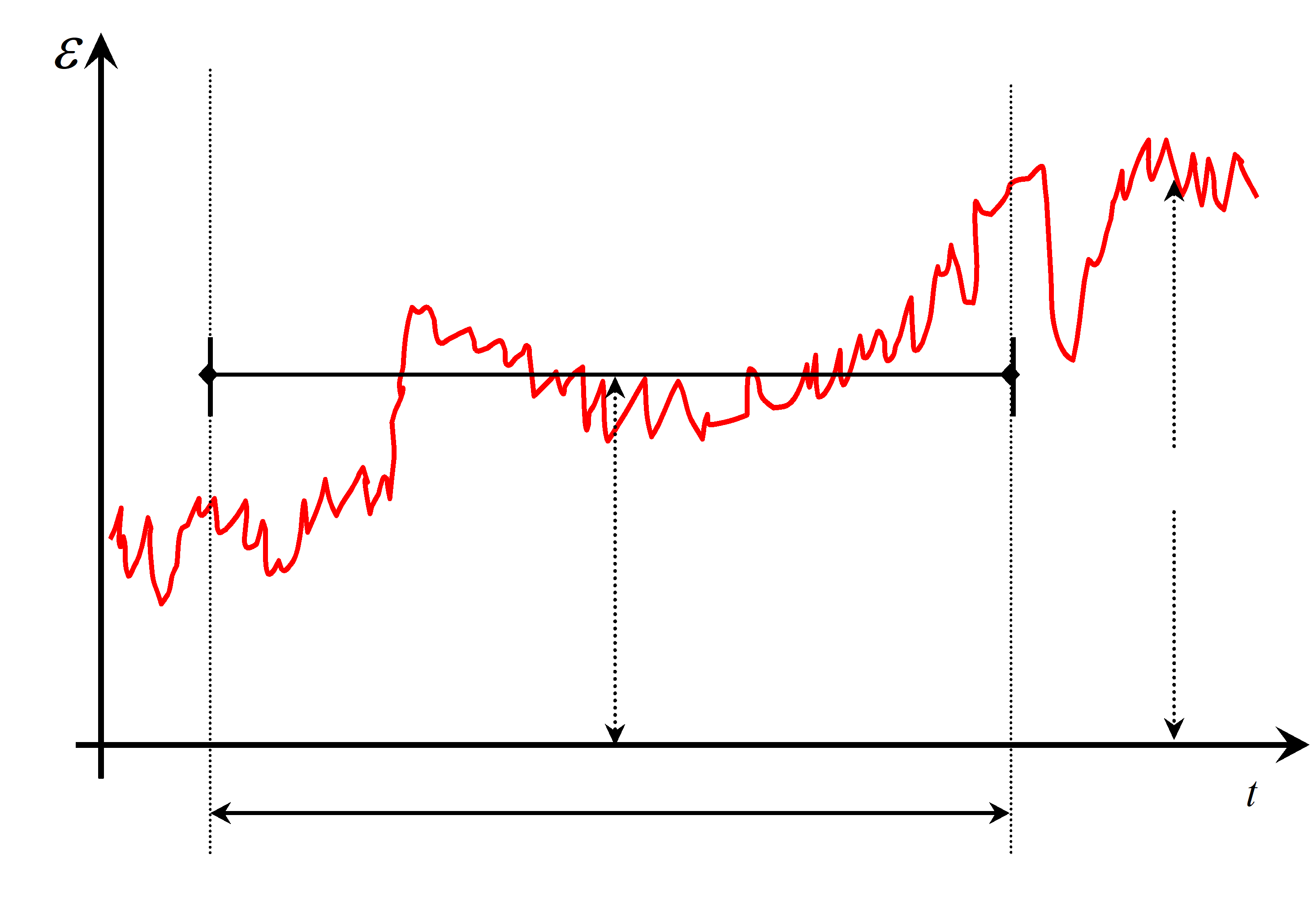Figure: AME, MME schematic definition

quaternion mean measurement error (MMEq)

MME in which the angular error is derived from the measured quaternion .

See note in B.5.4.

star mean measurement error (MMEs)

MME in which the angular error is derived from the measured star position

See note in B.5.5.

relative measurement error (RME)

the relative measurement Error (RME(t)) is defined as follows:

This is illustrated schematically in for a single axis rotation case in Figure B-2.

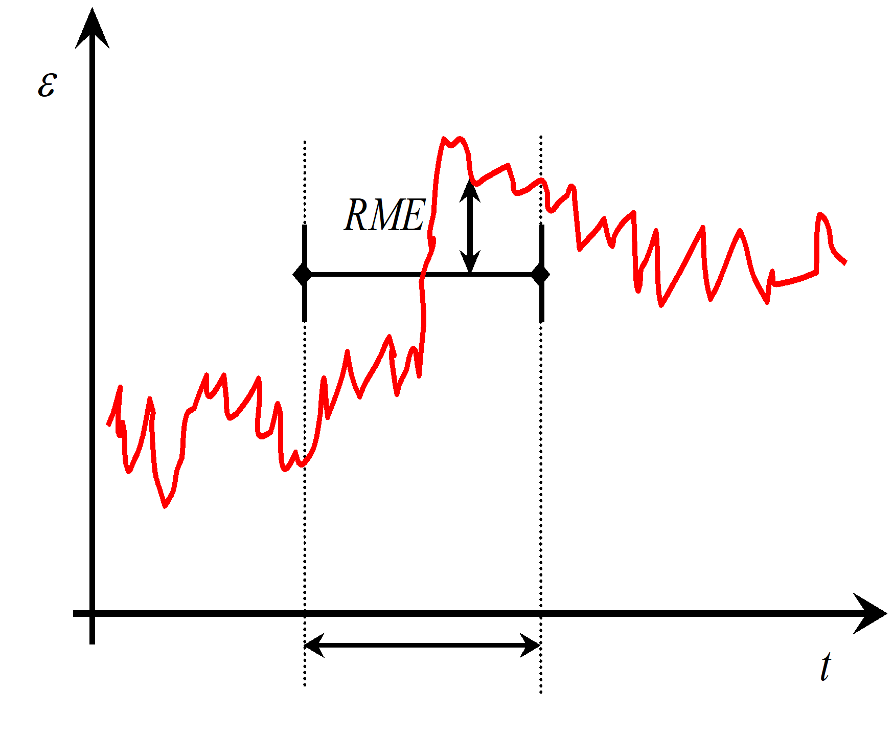Figure: RME Schematic Definition

quaternion relative measurement error (RMEq)

RME in which the angular error is derived from the measured quaternion

See note in B.5.4.

star relative measurement error (RMEs)

RME in which the angular error is derived from the measured star position

See note in B.5.5.

measurement drift error (MDE)

the measurement drift error (MDE(t)) is the difference between two successive mean measurement errors, separated by as follows:

where the lengths of the two successive intervals are set to identical values ; both intervals are contained in a longer interval with length

This is illustrated schematically in Figure B-3 for a single axis rotation case.

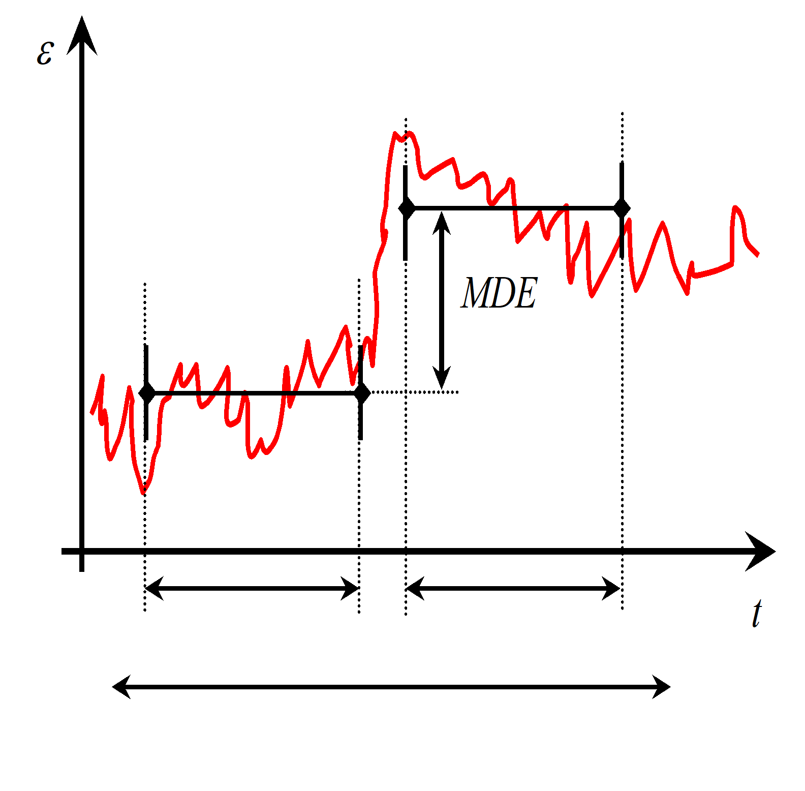Figure: MDE Schematic Definition

quaternion measurement drift error (MDEq)

MDE in which the angular error is derived from the measured quaternion .

See note in B.5.4.

star measurement drift error (MDEs)

MDE in which the angular error is derived from the measured star position

See note in B.5.5.

rotational error

Each of the metrics defined in clause B.5 is parameterized by 3 rotations around axis ‘j’ of a specific frame F. With respect to this frame, the rotational error Rj around each axis ‘j’ of the F frame is given by:

1 The rotational error is illustrated in Figure B-4.
2 The applicability of the specification formulation in terms of directional and rotational errors allows separate specification and performance statements relative to the direction of the sensor LOS and around the sensor LOS. This is useful since the performance in these 2 areas is typically significantly different for single optical head configuration and hence requires separate specification.

directional error

The directional error D(j) for axis ‘j’ is defined as the half-cone angle between the measured and reference position of axis ‘j’ and is given (for small rotation angles) by:

where ‘k’ and ‘l’ are the two axes perpendicular to axis ‘j’.

1 The directional error is illustrated in Figure B-4.
2 The applicability of the specification formulation in terms of directional and rotational errors allows separate specification and performance statements relative to the direction of the sensor LOS and around the sensor LOS. This is useful since the performance in these 2 areas is typically significantly different for single optical head configuration and hence requires separate specification.
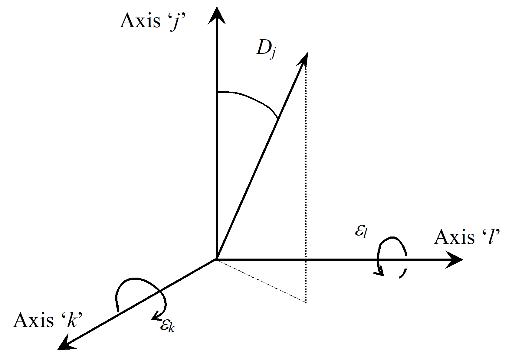Figure: Rotational and directional Error Geometry

Spatial errors

Some error contributors vary with the position of a star on the detector. These errors (e.g. field of view errors, pixel errors) can be tackled by spatial errors.

The mathematical expressions are the same as the ones presented in the clauses above, in which the time t is essentially replaced by a spatial position x.

For a more general domain variable, x, the indices can be redefined as follows:

Where is a specified region of parameter space and means that x lies within that region.

ANNEX(informative)Optional features of star sensors

Overview

This annex defines optional features or cabilities of star sensors. It follows the same structure as the clause 4 to allow for a direct link between requiremen and options.

Cartography

A sensor with cartography capability can have the following additional outputs: measurement of star magnitude of each detected star image.

The star images obtained need not be captured at the same instant in time.

Star tracking

1 Angular acceleration and jerk are supplied in the form of 3-dimension vectors giving the angular acceleration and jerk of the sensor BRF with respect to the IRF. These vectors are expressed in the sensor BRF.
2 In the case of external inputs coming from the spacecraft the star sensor supplier can indicate the minimum required accuracy for supplied data in order to properly switch into tracking.
A sensor with the star tracking capability can have the following additional outputs: measurement of star magnitude for each tracked star image.

Autonomous star tracking

The following additional inputs to launch tracking can be provided:
The angular acceleration and jerk of the sensor BRF with respect to the IRF, with their validity dates.
The accuracy of supplied inputs.

1 Angular acceleration and jerk are supplied in the form of 3-dimension vectors giving the angular acceleration and jerk of the sensor BRF with respect to the IRF. These vectors are expressed in the sensor BRF.
2 In the case of external inputs coming from the S/C the star sensor supplier can indicate the minimum required accuracy for supplied data in order to properly switch into tracking.
A sensor with the autonomous star tracking capability can have the following additional outputs: measurement of star magnitude for each tracked star image.

Autonomous attitude determination

A sensor with autonomous attitude determination can have the following additional outputs:
a measurement quality index or flag, estimating the accuracy of the determined attitude;
An inertial angular rate measurement projected on a sensor-defined reference frame;
a list of the star catalogue numbers for each star used in the determination;
the position of each star image with respect to a defined sensor reference frame;
measurement of star magnitude for each tracked star image.
the identification of the optical head(s) used for the attitude determination when multiple head configuration is used.

Autonomous attitude tracking

The following additional inputs to launch tracking can be provided:
the angular acceleration and jerk of the sensor BRF with respect to the IRF, with their validity dates;
the accuracy of supplied inputs including, in the case of attitude control, the accuracy around each axis of the sensor BRF.

1 Angular acceleration and jerk are supplied in the form of 3-dimension vectors giving the angular acceleration and jerk of the sensor BRF with respect to the IRF. These vectors are expressed in the sensor BRF.
2 In the case of external inputs coming from the S/C the star sensor supplier indicates the minimum required accuracy for supplied data in order to properly switch into tracking.
A sensor with autonomous attitude tracking capability can have the following additional outputs:
a measurement quality index or flag estimating the accuracy of the determined attitude;
an angular rate measurement around a sensor defined reference frame;
a list of the star catalogue numbers for each star used in the determination;
the position of each Star Image with respect to a defined reference frame;
the identification of the optical head(s) used for the attitude tracking when multiple head configuration is used.

Angular rate measurement

A sensor with angular rate measurement capability can have the following outputs:
a measurement quality index or flag, estimating the accuracy of the determined angular rate;
a validity index or flag, estimating the validity of the determined angular rate.

Types of star sensors

Star camera

A star camera can include the following additional capabilities: (partial) image download.

Star tracker

A star tracker can include the following additional capabilities:
autonomous star tracking;
(partial) image download.

Autonomous star tracker

An autonomous star tracker can include the following additional capabilities:
cartography;
star tracking;
autonomous star tracking (attitude acquisition with assisted attitude determination);
autonomous attitude tracking (with direct initialization);
angular rate measurement;
(partial) image download.

Summary

The specified minimum and additional cabilities for each type of sensor are summarized in Table C-1.
Table: Minimum and optional capabilities for star sensors

Type of sensor	Capabilities
Type of sensor	Cartography	Star Tracking	Autonomous Star Tracking	Autonomous Attitude Determination	Autonomous Attitude Tracking	Angular Rate Measurement	Partial Image Download
Star Camera	X						(X)
Star Tracker	X	X	(X)				(X)
Autonomous Star Tracker	(X)	(X)	(X)	X	X	(X)	(X)
Key: X = Mandatory, (X) = Optional Table Rows: type of star sensors; table columns: capability

ANNEX(informative)Performance metrics applied to star sensors

Overview

This annex discusses the performance metrics used to assess the performance of each star sensor capability. The definitions are derived from the ESA-NCR-502 (ESA Pointing Error Handbook) taking into account the specific case of star trackers:

the measurement errors are small;

the approximation of small Euler angles is possible.

Application to Star Sensor measurements

Overview

This clause applies the standard error metric definitions to the following types of Star Sensor measurement:

absolute rate measurements;

inertially referenced attitude, via a quaternion;

single star position measurement.

The distinction between quaternion and star position measurements is made.

Attitude quaternion measurements

The performance metrics AMEq, MMEq, RMEq and MDEq essentially cture the various frequency ranges of measurement error sources that contribute to the performance. These are summarized in Table D-1.

Table: Measurement error metrics

Metric	Lower Time Period of Contribution Variation	Upper Time Period of Contribution Variation
AMEq	0
MMEq (tMMEq)	MMEq
MDEq (tMDEq tOBS, MDEq)	MDEq	OBS, MDEq
RMEq (tRMEq)	0	RMEq

Typically, these performance metrics, with appropriate time period definitions, can be used to constrain the following commonly referenced types of measurement error:

Total measurement error – AMEq.

Bias errors - MMEq.

Long term errors and drifts - MDEq (with appropriate time definitions).

Short term errors - MDEq (with appropriate time definitions).

Noise errors, or Noise Equivalent Angle - RMEq.

Each of the metrics can be used to constrain rotational or directional errors as defined in clause B.5.14.

Star position measurements

The performance metrics , MMEs, RMEs and MDEs essentially cture the frequency ranges of measurement error sources that contribute to the performance. These are summarized in Table D-2.

Table: Star Position measurement error metrics

Metric	Lower Time Period of Contribution Variation	Upper Time Period of Contribution Variation
	0
MMES (tMMEs)	MMEs
MDES (tMDEs, tOBS, MDEs)	MDEs	OBS, MDEs
RMES (tRMEs)	0	RMEs

Typically, these metrics, with appropriate time period definitions, can be used to constrain the following commonly referenced types of measurement error:

Total measurement error – .

Bias errors - MMEs.

Long term and drift errors - MDEs (with appropriate time definitions).

Short term errors - MDEs (with appropriate time definitions).

Noise errors, or Noise Equivalent Angle - RMEs.

Each of the metrics can be used to constrain rotational or directional errors as defined in clause B.5.14.

ANNEX(informative)Statistics

Confidence level

Overview

The performances have a statistical nature, because they vary with time and from one realization of a sensor to another. Therefore, only an envelope of the actual performances can be specified and provided.

This envelope is the combination of an upper limit and a performance confidence level.

The performance confidence level indicates the proportion of the actual performances below the upper limit.

For example, the X absolute measurement error can be 10 arcsec with a performance confidence level of Pc = 95 %. This means that the actual errors from one sample to another are below 10 arcsec for 95 % of the cases.

Performance confidence level is usually 99,7 % (corresponding to a 3 sigma values for Gaussian distributions).

Accuracy on the confidence level

The verification of the specifications can only be done on a limited set of samples of the whole statistical population:On a limited time span

On a limited number of sensors

The larger the set of samples, the better the knowledge on the performance confidence level (Pc).

This implies that the actual confidence level is not perfectly known, but is estimated with a certain accuracy P, also called accuracy on the confidence level.

This qualitative notion can be mathematically expressed by using:

The performance confidence level (Pc): it applies to the performances quoted by manufacturers and specified by customers (usually as 3 sigma values).

And the estimation confidence level. It applies to the estimation of the performance confidence level (defined above). It represents the confidence that the sample is representative of the overall ensemble.

If not specified, confidence level means performance confidence level, and is denoted Pc in this document.

The confidence estimation accuracy ( ) being fixed, the minimum number of samples (N) depends on the estimation confidence level.

For an estimation confidence level 95%, then the minimum number of samples is given by . It means that if the number of samples is larger than N, then the actual confidence level lies in the range in 95 % of the cases

For an estimation confidence level 99,7 %, then the minimum number of samples is given by . It means if the number of samples is larger than N, then the actual confidence level lies in the range in 99,7 % of the cases

Further details can be found in clause B.2.

E.g. If the performance confidence level is 99,7 % and the accuracy is P = 0,1 %, then at least 11964 samples are considered to actually demonstrate that the actual performance confidence level is between 99,6 % and 99,8 % (i.e. it is known with an accuracy of 0,1 %), with a confidence of 95 %.

Mathematical derivation

N samples of a random variable x from a probability distribution function p(x) are considered. Denote the actual performance confidence level of interest by , with true value . Then the number of samples within the set N lying below is sampled from a binomial distribution with mean and variance given by:

The estimate of the performance confidence level at is given as follows:

Therefore the mean and variance of the estimate of the performance confidence level is given by:

(i.e. the mean value of the estimate is the actual value)

Now, let be the estimation confidence accuracy, such that the actual value Pc of the performance confidence level lies in the range , with a given estimation confidence level.

The variations of are supposed to follow a Gaussian distribution. With this assumption, if the estimation confidence level is set to 95 %, (which corresponds to ), then the minimum number of samples in the set N to be calculated is:

For a 99,7 % estimation confidence level on , the formula becomes , because 99,7 % corresponds to a 3 sigma value for a Gaussian distribution.

More generally, for a nC-sigma estimation confidence level of a Gaussian distribution.

For example, if the performance confidence level on the error is 99,7 % and the accuracy is P = 0,1 %, then at least 11964 samples are the minimum number of samples used to actually demonstrate that the actual confidence level is between 99,6 % and 99,8 % (i.e. it is known with an accuracy of 0,1 %), with an estimation confidence level of 95 %.

Minimum number of runs with no failure

The previous clause focuses on the minimum number N of simulations to run to demonstrate the performances within a given performance confidence level and a given accuracy on the estimation confidence level.

Another approach, more efficient from the implementation point of view, is to consider the number Nt of simulations to run if no failure occurs to demonstrate the same performances. In this context, a failure is a simulation in which the performance level to be demonstrated is exceeded.

This number of simulations Nt is usually much smaller than N, which makes the approach more appropriate.

E.g. if the requirement is specified at 99,73 %, then the number of samples to estimate this performance confidence level with a 95 % estimation confidence of the real value being within ±0,1 % of the estimate is N = 11964. However assuming no failures are seen, only Nt =1108 runs are required to prove that the probability of failure is <0,27 % to a 95 % estimation confidence level.

Suppose that we have a specification P(x<xmax)>Pmin, with some statistical interpretation. This means that for the system to meet its specification, in any given trial the probability of having x < xmax is at least Pmin. Equivalently, the probability of having a failure (x>xmax) in any given trial is less than Pfmax = 1-Pmin.

Given a campaign with Nt runs, of which nf of these are failures. Assuming that the real underlying probability of failure (not known to the experimenter) is Pf, then the probability of observing nf failures in Nt trials is given by the binomial formula:

The relation with the normalization condition yields:

If there is no a-priori information about the probability of failure, then the most conservation approach is to assume that the probability of failure is uniformly distributed between 0 and 1:

This yields

Then, for a given number of observed failures nf the probability distribution of Pf is found to be:

If the probability of failure is less than some value Pfmax, the specification is met. (This is equivalent to a minimum probability of not failing the specification.) Given nf failures in trials, the confidence of the specification actually being met (i.e. of Pf really being less than Pfmax) is:

where βinc is the incomplete beta function given by:

This function is available in usual engineering tools.

Using this formula, it is possible to work out the minimum number of runs in order to meet the specifications with a given probability to a given performance confidence level.

Table E-1 gives numerical plications for various cases.

Table: Minimum number of simulations to verify a performance at performance confidence level PC to an estimation confidence level of 95 %

Performance confidence level PC	Minimum number of runs for number of observed failures Nfail
Performance confidence level PC	Nfail = 0	Nfail = 1	Nfail = 2	Nfail = 3
68 %	7	12	17	21
95 %	58	92	123	152
99,73 %	1108	1755	2329	2869
NOTE: ‘failure’ in this context means violation of the specified bound, x > xmax.

There is no equivalence to the estimation confidence accuracy introduced in clause B.1.3. It means that the estimation confidence level is at least the level specified (e.g. 95 % in the table above).

Statistical interpretation of measurement error metrics

Each of the metrics defined in clause B.5 is typically specified and used with an associated confidence level.

Any performance metrics depends on several variables:

the time t;

the realization of the sensor (involving the manufacturing process);

the observation conditions in which the performances are obtained (e.g. angular rate applied on the sensors, orientation with respect to the celestial vault).

As it is not possible to build a representative sample set of sensors, the notion of statistical ensemble is used. A statistical ensemble of sensors is defined as a collection of sensors representative of the manufacturing process, in which not all sensors are necessarily built.

Because a metrics depends on several variables, there are several ways to interpret a specification and its confidence level:

Temporal interpretation

The worst case combination of sensors and observations is considered.

The worst-case sensor/observation combination is defined as the worst-case sensor observing the worst-case direction in the celestial vault under the worst-case observation conditions. The worst-case direction is the one leading to the worst performance of the sensor. It is related to the worst distribution of stars over the star sensor field of view, taking into account embedded algorithms and catalogues.

The performances are established with respect to time.

The specification metric is ‘less than S for n% of the time for a worst-case sensor/observation from a statistical ensemble of sensors/observations’.

Ensemble interpretation

A statistical collection of sensors is arbitrarily chosen.

A given set of observations is arbitrarily chosen.

The time is set to the worst case time, i.e. when the performances obtained for a given sensor and observation are worst.

The specification metric for this type of variability is ‘less than the level S in confidence level n% of a statistical ensemble of sensors/observations for the worst-case time’.

Mixed interpretation

The mixed interpretation combines the ensemble and temporal variation to capture the error variability both over time and across the ensemble.

The specification metric for this type of variability is ‘for a random sensor/observation from the statistical ensemble, and at a random time, the metric is less than S with a probability of n%’.

For a generic measurement error source with an amplitude and a time variation, the ensemble interpretation gives the distribution of the error amplitude over the statistical ensemble of sensors/observations, while the temporal interpretation covers the error variation over time for the worst-case amplitude.

For the AME, RME and MDE metrics defined in clause B.5, the statistical interpretation can in principle be ensemble, temporal or mixed. However, the nature of the MME metric means that only an ensemble interpretation is propriate. Specific identification of the interpretations to be used in this specification is given in Annex D.

ANNEX(informative)Transformations between coordinate frames

Transformations between any two co-ordinate frames, A and B can be described by the transformation matrix which transforms the components of a vector from ‘B’ frame to ‘A’ frame:

where are the components of the vector in the ‘A’ frame, and are the components of the same vector in the ‘B’ frame.

The discrepancy between both frames ‘A’ and ‘B’ is defined by 3 Euler angles around 3 distinct axes. In this Standard, the rotations are always small, therefore the order of the rotations is not important and these rotations can be taken to be rotations around the X-, Y- and Z-axes of either frame.

The transformation is simply:

where , and are the 3 small rotations respectively around X, Y and Z axes transforming the ‘B’ frame into the ‘A’ frame.

The discrepancy between both frames ‘A’ and ‘B’ is:

The discrepancy is a function of the time.

The performances of star sensors are measured by plying the metrics defined in Annex D to this vector .

For star sensors, this vector typically represents the angular errors between a measured quantity and its actual value.

E.g. With ‘A’ frame being the actual star sensor frame and ‘B’ frame being the measured star sensor frame, then represen the measurement errors of the star sensor (see Figure F-1).

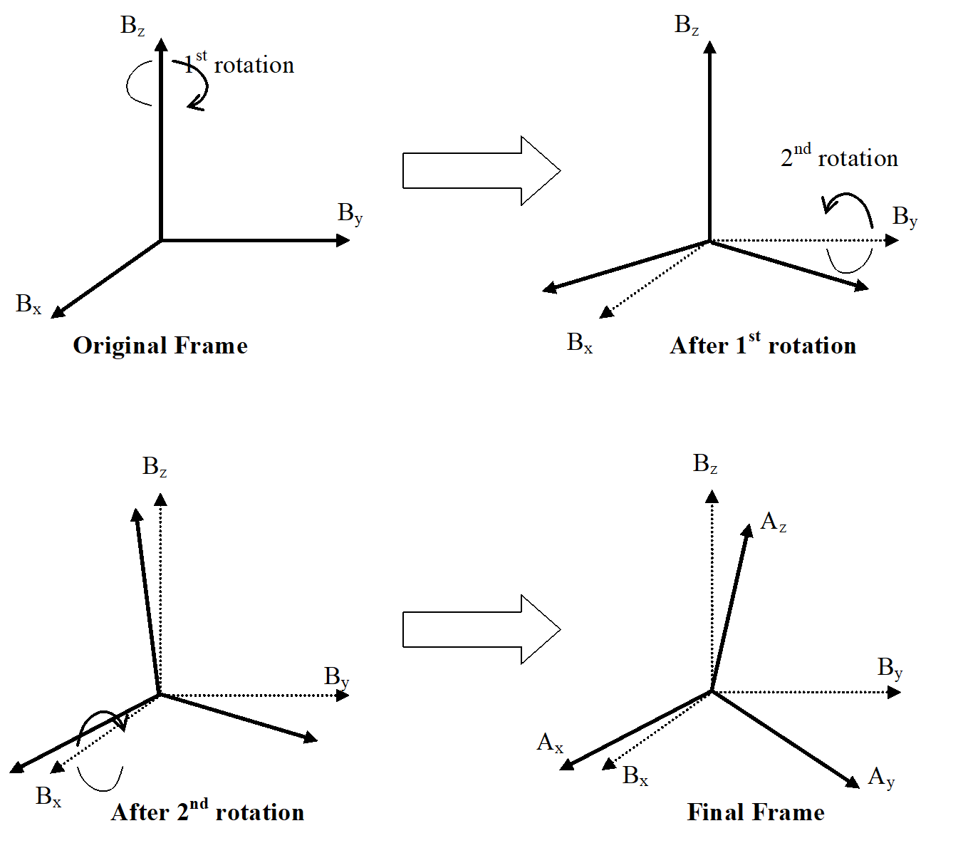Figure: Angle rotation sequence

In this case the 3-axis Euler rotation parameterization corresponds to rotations around the B-frame axes.

The separation of two frames A and B, defined in the ESA Pointing Error Handbook and written as is defined as:

This function represents the discrepancy between the two frames and is used to measure the star sensor performances.

ANNEX(informative)Contributing Error Sources

Overview

This annex links the error contributors to the definitions derived from the ESA-NCR-502 (ESA Pointing Error Handbook). The traditional contributors and performances are compared with generalized error with respect to the corresponding correlation time  given for each contributor.

Table: Contributing error sources

Error contributors

Comments

Bias

- on-ground calibration residual

- launch-induced misalignment (vibrations, depressurization, gravity…)

BRF vs MRF misalignment due to after-launch ageing

MME ( = infinite)

MME ( = life time)

Thermo elastic error

BRF vs MRF stability due to :

- stabilized optical head temperature

- gradient caused by conductive and radiative effects

MDE ( = once the thermal scenario is known.)

 = correlation length

obs = observation length

FOV spatial errors
- Point Spread Function variability across the FOV

- residual of calibration of focal length (including its temperature sensibility) and optical distortions (including chromatism)

- residual of aberration of light in case where it is corrected at quaternion level and not at star level

- CCD CTE effect (including its degradations due to radiations)

- catalogue error (including star proper motion and parallax)

The amplitude of these errors are independent of the rate.

The  is assessed by the supplier in the angular domain.

There is a need to get the figures for several values. The use of autocorrelation function of spatial error is recommended.

MDE ( to be described )

Can be converted by the user in time domain depending on the specific application. using angular rate

Pixel spatial errors
- detector non uniformity (FPN, DSNU (DS(T), radiation, integration time…), PRNU(straylight, star signal photonic noise)…)

- centroiding (rate dependent)

The  is assessed by the supplier in the angular domain.

Can be converted by the user in time domain depending on the specific application using angular rate.

MDE ( linked to pixel FOV)

Temporal noise
- star signal shot noise depending on star signal (Star Magnitude, exposure time, optical contamination, transmission loss, defocus, rate…)

- background signal shot noise (straylight level, detector temperature…)

- read-out noise

- quantification noise

- datation noise

RME ( =0 or less than the sample time)

Aberration of light or residual of aberration of light correction if corrected at star level

MDE ( =TBD by user)

residual of aberration of light correction if corrected at star level

As this error is very deterministic, it is possible to correct it inside the star tracker - supposing that the velocity information is given to the star tracker. A few cases are quoted:

1) a correction is performed for every star direction,

2) a unique correction is performed globally for a unique direction (example: line of sight, or barycentre of the measured stars) and applied on the quaternion or on each star measurement,

3) a correction is performed only for the Earth / Sun velocity,

4) no correction is performed.

Depending on the correction, the error residual is:

- a FOV spatial error if the correction is performed globally (case 2)

- an orbital error in the case 3 (depending also on the attitude of the spacecraft)

- a long term error (one year) + orbital error for the case 4.

ANNEX(informative)Example of data sheet

Introduction

The data sheet in Figure H-1 shows an example of data sheet for autonomous star tracker.

The fields that can be filled in are identified in an italic font.

The example values filled in are just for formatting purposes and do not relate to an existing star sensor.

Rules applied

The following rules have been plied to provide the data sheet in Figure H-1:

use of the content of the example data sheet proposed in the “Star Sensor Terminology and Performance Specification Standard”, issue 1 and addition of some key items. (first version of the present document issued by ESA studies);

the data sheet has been limited to one page of format A4 but is not mandatory.

Figure: Example of detailed data sheet

Bibliography

ECSS-S-ST-00	ECSS system – Description, implementation and general requirements
ESA-NCR-502	ESA Pointing Error Handbook